Welcome!
This site contains lecture notes, tutorials, and assignment instructions for COMP 4630: Machine Learning. Use the sidebar on the left to view the material, and if you notice a problem, please report an issue at the GitHub repo.
Sometimes I’ll write stuff on the board. You can find a version of my scribbles here, which I’ll try to keep more or less up to date.
Lecture 1: Data Exploration
 HTML Slides
 PDF Slides
Welcome to Machine Learning!
COMP 4630 | Winter 2026 Charlotte Curtis
What is this course about?
- Continuing the supervised/unsupervised learning algorithms from COMP 3652, with a focus on Neural Networks
- First half: the history, theory, and math behind neural networks
- Second half: applications of NNs in computer vision, natural language processing, and more
This is not (just) a course on building models using libraries like TensorFlow or PyTorch, it is a course on understanding the theory
How did I get involved with ML?

What do you want to learn about ML?
❓
Grade Assessment
| Component | Weight |
|---|---|
| Assignments | 3 x 10% |
| Midterm (theory) exam | 20% |
| Journal club | 10% |
| Final project | 40% |
Bonus marks may be awarded for substantial corrections to materials, submitted as pull requests
Course materials repo: https://github.com/mru-comp4630/w26 Rendered at: https://mru-comp4630.github.io/w26/
Textbooks and other readings
Primary Textbook:
- Hands on Machine Learning with Scikit-Learn and [Tensorflow/PyTorch]
- Associated GitHub repo (Tensorflow)
- Associated GitHub repo (PyTorch)
More mathy details:
Journal club list: on D2L under “Course Info” (requires MRU library login)
Generative AI policy
- Yes, AI can do a lot of what I’m asking for in this course
- No, I do not want to read about what AI “thinks”
- ❓ What do you think is an appropriate use?
Machine Learning Project Checklist
Appendix A of the hands-on textbook
- Frame the problem and look at the big picture.
- Get the data.
- Explore the data to gain insights.
- Prepare the data to better expose the underlying data patterns to Machine Learning algorithms.
- Explore many different models and short-list the best ones.
- Fine-tune your models and combine them into a great solution.
- Present your solution.
- Launch, monitor, and maintain your system.
1. Look at the big picture
Example Dataset: California housing prices (1990)
❓ Discussion questions:
- How does the company expect to use and benefit from this model?
- What is the current solution?
- What kind of ML task is this?
- What kind of performance measure should we use?
Where we left off on Wednesday, January 7
First, some stuff about assessments
- Assignment 1
- Journal club guidelines
- Example of a math-heavy paper
- Additional references for papers:
2. Get the data
For this class, we’ll use readily available datasets. Some sources are:
- UCI Machine Learning Repository
- Kaggle
- Google Dataset Search
- Various Government open data portals (e.g. Calgary, Alberta, Canada)
After fetching the data, set aside a test set and don’t look at it.
“Get the data” can often be a huge task in itself!
2a. Set aside a test set
❓ Discussion questions:
- Why do we need an independent test set?
- Avoid data snooping bias
- Relevant XKCD
- Why would we use a random seed?
- What is naive about simply selecting a random sample?
- What else could we do?
- What is stratified sampling?
Side tangent: Sampling bias
- Simple example: assume 80% of population likes cilantro
- Goal: ensure our sample is representative of the population,
The binomial distribution can be used to model the probability of choosing people who like cilantro from total participants:
Side tangent: Sampling bias continued
is the probability mass function, and the corresponding cumulative distribution function is just the sum up to :
Suppose we randomly sample 100 people. What is the probability of fewer than 75 or more than 85 cilantro lovers?
This is also my excuse to review some probability theory and notation
3. Explore the data
❓ Discussion questions:
- What do you notice about the data?
- Do the values make sense for the labels?
- Is the scale of the features comparable? Does this matter?
- What possible biases might be present in the data?
3a. Look for correlations
The Pearson correlation coefficient is a measure of the linear correlation between two variables and (commonly denoted as ):
where and are the sample means of and , respectively.
- What do correlations of 0, 1, and -1 mean?
- What are some limitations of Pearson correlation?
Where we left off on Monday, January 12
4. Prepare the data
General goals:
- Handle missing data, and maybe outliers
- Drop irrelevant features
- Combine features using domain knowledge
- Apply various transformations (e.g. scaling, encoding)
- Apply scaling when necessary
4a. Handling missing data
In the book 3 options are listed to handle the NaN values:
housing.dropna(subset=["total_bedrooms"], inplace=True) ## option 1
housing.drop("total_bedrooms", axis=1)                  ## option 2
median = housing["total_bedrooms"].median()             ## option 3
housing["total_bedrooms"].fillna(median, inplace=True)
❓ Discussion questions:
- What is each option doing?
- What are the pros and cons of each option?
- Which one should we choose?
4b. Handling non-numeric data
Most of the math in ML algorithms is based on numbers, so we need to convert text and categorical attributes to numbers. This is called encoding.
❓ Discussion questions:
- Which columns of our data are categorical?
- What methods could we use to convert them to numbers?
- What are the assumptions about the various encoding methods?
4c. Scaling the data
Many ML algorithms don’t like features with vastly different scales. Common scaling methods are min-max scaling and standardization.
Important: scaling is computed on the training set and applied to the validation and test sets - they are not scaled independently!
❓ Discussions questions:
- What are the bounds of each method?
- Which method is more affected by outliers?
- How would you decide which method to use?
4e. Standardization details
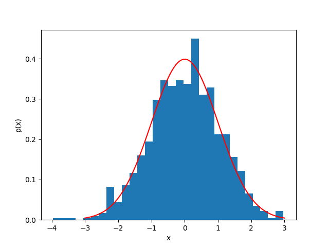
A general Gaussian distribution is given by:
where is the mean and is the standard deviation. The standard normal distribution is a special case where and , reducing the equation to:
4f. Other transformations
- Log transformation: useful for data that is heavily skewed
- Also square root, squaring, etc.: try to remove heavy tails
- Feature engineering: combining features to create new ones
- Binning: turning continuous data into discrete categories
- Possibly using K-means clustering
- Relies on domain knowledge
- Best to create a transformation pipeline and apply it to the data rather than saving the transformed data
Coming up next
- Math review:
- Linear algebra
- Differential calculus
- Statistics
- A brief introduction to vector calculus
Lecture 2: Math Review
Math review
COMP 4630 | Winter 2026 Charlotte Curtis
Math review
- MATH 1203: Linear algebra
- MATH 1200: Differential calculus
- MATH 2234: Statistics
Further reading:
- Linear algebra: notebook, deep learning book
- Calculus: notebook
Linear algebra
Vectors are multidimensional quantities (unlike scalars):
A common vector space is , or the 2D Euclidean plane. Example:
Vector operations
- Addition:
- Scalar multiplication:
- Dot product: (yields a scalar)
- Can be thought of as the projection of one vector onto another, or how much two vectors are aligned in the same direction
Vector norms
- The norm of a vector is a measure of its length
- Most common is the Euclidean norm (or norm):
- You might also see the norm, particularly as a regularization term:
Useful vectors
- Unit vector: A vector with a norm of 1, e.g. ,
- Normalized vector: A vector divided by its norm, e.g.
- Dot product can also be written as
Yes, a normalized vector is also a unit vector, main difference is in context and notation
Matrices
A matrix is a 2D array of numbers:
Notation: Element is in row , column , also written as .
Rows then columns! matrix has rows and columns
Matrix operations
- Addition: element-wise if dimensions match.
- Scalar multiplication: just like vectors
- Matrix multiplication: where the elements of are:
- Multiply and sum rows of with columns of
- Usually,
Matrix multiplication examples
Matrix times a matrix:
Matrix times a vector:
Where we left off on January 14
Matrix transpose
-
Transpose: swaps rows and columns
-
Inverse: just as , , where is the identity matrix
Not every matrix is invertible!
Calculus: Notation
The derivative of a function is represented as:
The second derivative is denoted:
and so on.
Differentiability
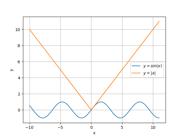
For a function to be differentiable at a point , it must be:
- Defined at
- Continuous at
- Smooth at
- Non-vertical at
Select rules of differentiation
| Function | Lagrange | Leibniz | |
|---|---|---|---|
| Constant | |||
| Power | with | ||
| Sum | |||
| Exponential | |||
| Chain Rule |
Chain rule example
-
Find for
-
Now, let, , where . What is ?
Partial derivatives
For a scalar valued function , there are two partial derivatives:
These are computed by holding the “other” variable(s) constant. For example, if , then:
A brief introduction to vector calculus
Putting together partial derivatives with vectors and matrices we get:
Scalar-valued :
Vector-valued :
Most of the time we’ll just be working with the gradient
Statistics: Notation
- A random variable is a variable that can take on random variables according to some probability distribution
- may take on discrete (e.g. dice rolls) or continuous (e.g. age) values
- or for the random variable and or for a specific value
- for a a discrete distribution and for continuous
- and
Some textbooks/papers/websites use different notation!
Discrete random variables
- A discrete probability mass function describes the probability of taking on a specific value
- Example: for a balanced 6-sided die,
- You can add together probabilities, e.g.
- and for any valid distribution
Continuous random variables
- A continuous probability density function gives the probability of being in some tiny interval given by
- Example: the uniform distribution, for
- for any specific value
- Need to integrate to get a concrete value, e.g.
- and for any valid distribution
Expectation and variance
- The expectation or expected value is its average value
- and
- More generally, for any function :
- The variance describes how much the values vary from their mean:
Multiple random variables
- Joint probability is the probability of and occurring together
- Conditional probability is the probability that takes on value given that has already happened
- In general,
- For independent variables,
Covariance
- The covariance between and gives a sense of how linearly related they are and how much they vary together:
- Related to correlation as
- The covariance matrix of a random vector is a square matrix where the element is the covariance between and
- The diagonal of the covariance matrix gives
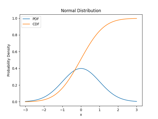
The Normal distribution
Good “default choice” for two reasons:
- The central limit theorem shows that the sum of many ( ish) independent random variables is normally distributed
- Has the most uncertainty of any distribution with the same variance
We can’t easily integrate , so numerical approximations are used
Coming up next
- Training (regression) models
- Linear regression
- Gradient descent
- References and suggested reading:
- Scikit-learn book:
- Chapter 4: Training Models
- Deep Learning Book
- Section 5.1.4: Linear Regression
- Scikit-learn book:
Lecture 3: Training models
Training Models with Regression and Gradient Descent
COMP 4630 | Winter 2026 Charlotte Curtis
Overview
- Linear Regression and the Normal Equation
- Gradient Descent and its various flavours
- References and suggested reading:
- Scikit-learn book:
- Chapter 4: Training Models
- Deep Learning Book
- Section 5.1.4: Linear Regression
- Scikit-learn book:
Linear Regression
Unlike most models, linear regression has a closed-form solution called the Normal Equation:
where
- are the weights of the model minimizing the cost function
- is the vector of target values
- is the design matrix of feature values
As usual, different sources use different notation, e.g. or instead of .
Consider the 1-d case:
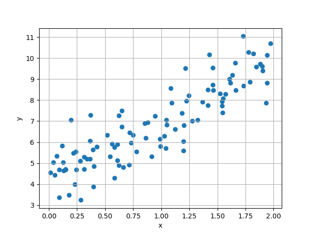
we want the values of and that minimize the Mean Square Error between the actual and predicted values:
Solving for and
Math time!
Solving for and
After some algebraic gymnastics, we get:
where and are the means of the and values, respectively.
Expanding to matrix form
Instead of the scalar or even vector , it’s common to use a design matrix to represent the feature values:
where each row is an instance (sample) and each column is a feature.
The first column is all ones, representing the bias term
Back to the linear regression problem…
-
We can rewrite the estimate in matrix notation:
-
The MSE can be written as:
where we’ve used the trick of substituting
:abacus: Find the gradient of the MSE w.r.t , set it to zero, and solve for
Properties of matrices and their transpose
The following properties are useful for solving linear algebra problems:
Additionally, any matrix or vector multiplied by is unchanged.
The Normal Equation
We made it! The Normal Equation is again:
- No optimization is required to find the optimal
- Limitations:
- must be invertible and small enough to fit in memory
- The computational complexity is (at least)
- Even in linear regression problems, it is common to use gradient descent instead due to these limitations
Gradient Descent
The goal of gradient descent is still to minimize the cost function, but it follows an iterative process:
-
Start with a random
-
Calculate the gradient for the current
-
Update as
-
Repeat 2-3 until some stopping criterion is met
where is the learning rate, or the size of step to take in the direction opposite the gradient.
Stochastic Gradient Descent
- Standard or batch gradient descent uses the entire training set to calculate the gradient for each instance at every step
- Stochastic Gradient Descent uses a single random instance at each step:
- Start with a random
- Pick a random instance (row in the design matrix)
- Calculate the gradient for the current and
- Update as
- Repeat 2-4 until some stopping criterion is met
Mini-batch Gradient Descent
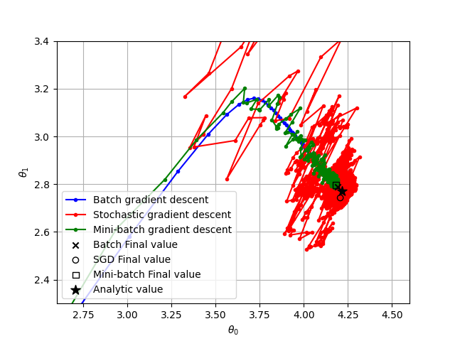
- Mini-batch gradient descent uses a random subset of the training set
- Less chaotic than stochastic, but faster than batch
- Most common type of gradient descent used in practice
Gradient Descent Hyperparameters
- The learning rate - size of step taken
- No rule that it needs to be constant! A simple learning schedule is to decrease over time, e.g.: where is the current iteration and and are hyper-parameters
- For mini-batch, the batch size is another hyper-parameter
- The number of epochs, or times to process the entire training set
Stopping Criteria
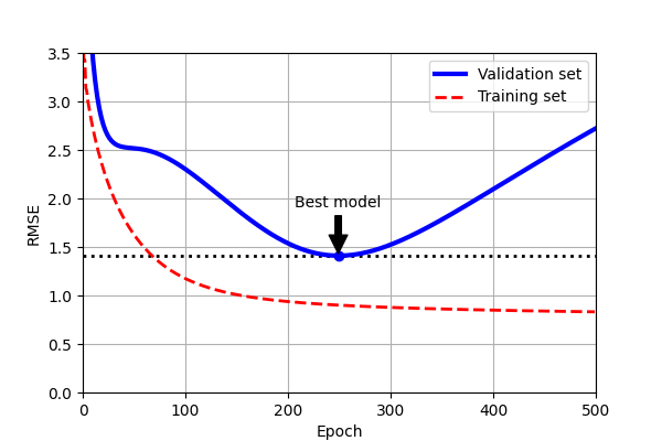
- The simplest stopping criterion is to set a maximum number of epochs
- Early stopping is another option:
- Evaluate on a validation set at regular intervals
- Stop when the validation error starts to increase
- The comparison between training and validation performance can also help prevent overfitting
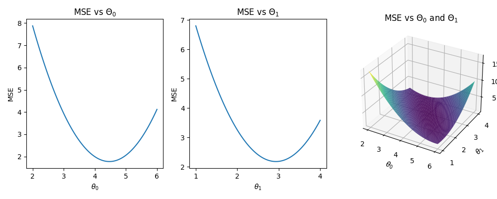
Loss functions
-
The loss function is the function being minimized by gradient descent
-
MSE is convex and guaranteed to have a single global minimum, but many other loss functions have multiple local minima
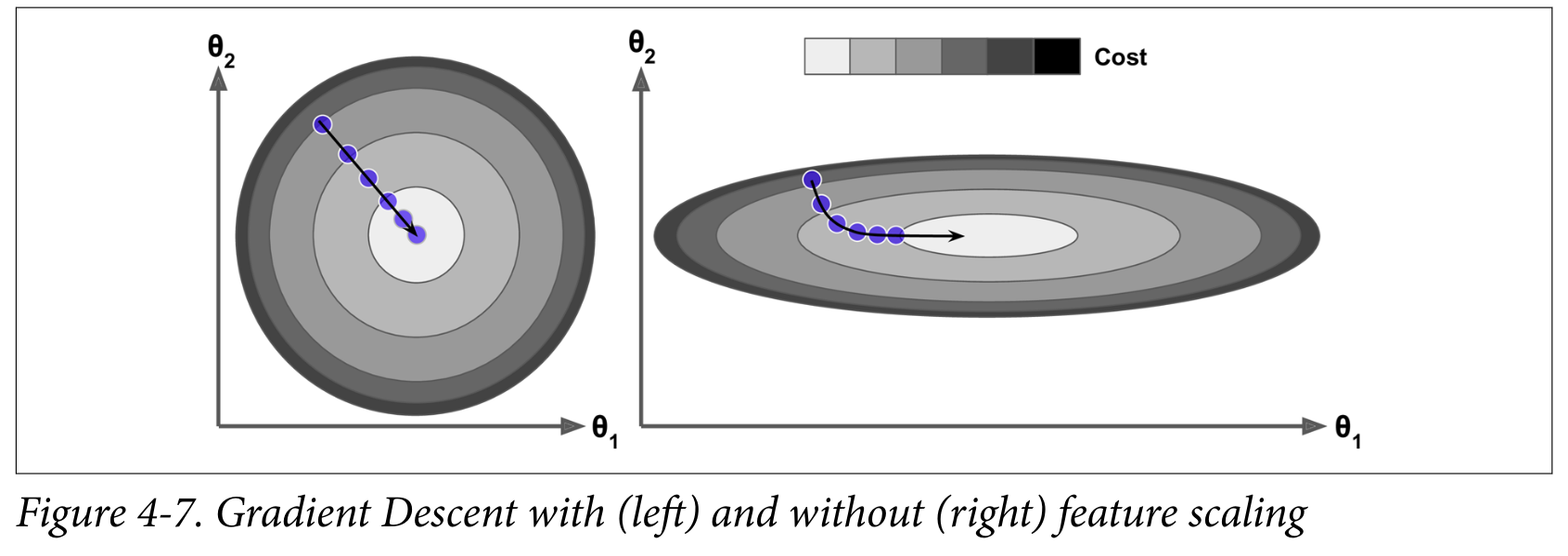
-
The relative scale of the features can affect the convergence:
Higher-order Polynomials
- Higher order polynomials can be solved with the Normal Equation as well:
- Just include the higher order terms in
- This is still a linear regression problem because the coefficients are linear!
- Risk of overfitting the data
- Easy way to regularize: drop one or more of the higher order terms
Regularization
- If the model fits the training data too well, but doesn’t generalize to new data, it is overfitting
- Regularization imposes additional constraints on the weights
- Example: Ridge Regression adds a term to the loss function: where is the regularization parameter
- The regularization term is only added during training, not evaluation
Note: the term cost function is often used instead of loss function
Logistic regression and beyond
Logistic regression is a binary classifier that uses the logistic function (aka sigmoid function) to map the output to a range of 0 to 1:
We can then minimize the log loss or cross-entropy loss function:
where is the probability that instance is positive.
The gradient of the log loss ends up being:
- There is no (known) analytical solution this time, but we can still use gradient descent!
- In this case it’s still convex, so we don’t have to worry about local minima
- In general, for a loss function to work with gradient descent, it must be:
- Continuous and
- Differentiable
- … at the locations where you evaluate it
Next up: Backpropagation!
Lecture 4: Backpropagation
Backpropagation
COMP 4630 | Winter 2026 Charlotte Curtis
Overview
- A brief review of the history of neural networks
- Neurons, perceptrons, and multilayer perceptrons
- Backpropagation
- References and suggested reading:
- Scikit-learn book: Chapter 10, introduction to artificial neural networks
- Deep Learning Book: Chapter 6, deep feedforward networks
The rise and fall of neural networks

In between each era of excitement and advancement there was an “AI winter”
Model of a neuron
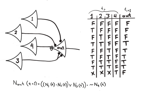
- McCulloch and Pitts (1943)
- Neuron as a logic gate with time delay
- “Activates” when the sum of inputs exceeds a threshold
- Non-invertible (forward propagation only)
Threshold Linear Units (TLUs)
- Linear I/O instead of binary
- Rosenblatt (1957) combined multiple TLUs in a single layer
- Physical machine: the Mark I Perceptron, designed for image recognition
- Criticized by Minsky and Papert (1969) for its inability to solve the XOR problem - first AI winter
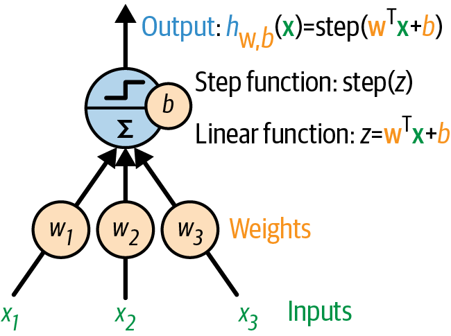
A single threshold logic unit (TLU)
Image source: Scikit-learn book
Training a perceptron
-
Hebb’s rule: “neurons that fire together, wire together”
where = input, = output
-
Fed one instance at a time,
-
Guaranteed to converge if inputs are linearly separable
-
:abacus: Simple example: AND gate
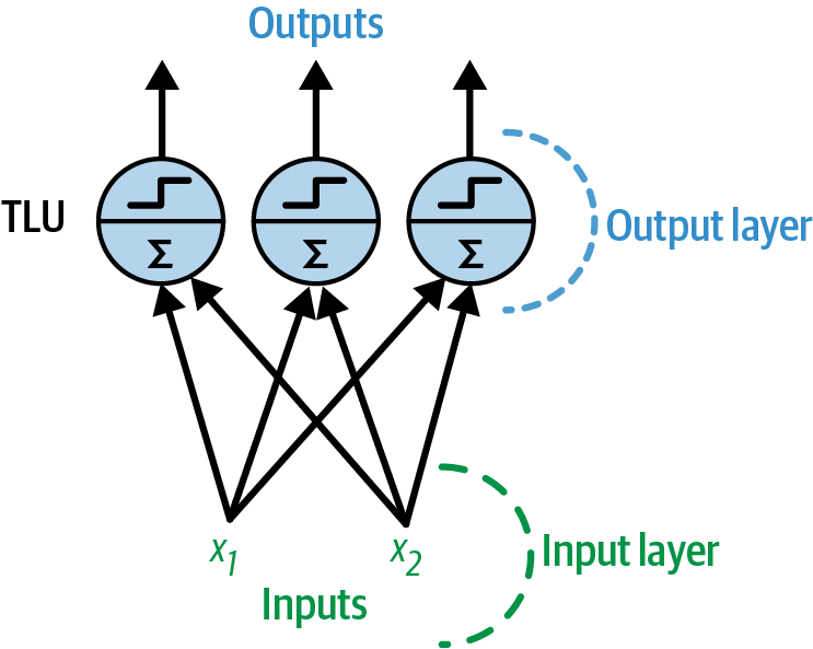
A perceptron with two inputs and three outputs
Image source: Scikit-learn book
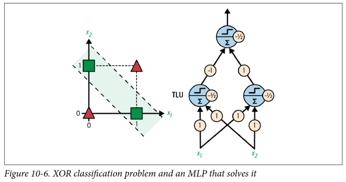
Multilayer perceptrons (MLPs)
-
If a perceptron can’t even solve XOR, how can it do higher order logic?
-
Consider that XOR can be rewritten as:
A xor B = (A and !B) or (!A and B) -
A perceptron can solve
andandorandnot… so what if the input to theorperceptron is the output of twoandperceptrons?
A solution to XOR
Backpropagation
- I just gave you the weights to solve XOR, but how do we actually find them?
- Applying the perceptron learning rule no longer works, need to know how much to adjust each weight relative to the overall output error
- Solution presented in 1986 by Rumelhart, Hinton, and Williams
- Key insight: Good old chain rule! Plus some recursive efficiencies
Training MLPs with backpropagation
-
Initialize the weights, through some random-ish strategy
-
Perform a forward pass to compute the output of each neuron
-
Compute the loss of the output layer (e.g. MSE)
-
Calculate the gradient of the loss with respect to each weight
-
Update the weights using gradient descent (minibatch, stochastic, etc)
-
Repeat steps 2-5 until stopping criteria met
Step 4 is the “backpropagation” part
Example: forward pass
- With a linear activation function:
- In summation notation for a single sample:
- In this case,

and
Example: calculate error and gradient
- We never picked a loss function! Let’s assume we’re using MSE
- For a single sample: with the added for convenience
- The goal is to update each weight by a small amount to minimize the loss
- Fortunately, we know how to find a small change in a function with respect to one of the variables: the partial derivative!
Recursively applying the chain rule
-
Weights in the second layer (connecting hidden and output):
-
For the first layer (connecting inputs to hidden): where is the output of the hidden layer
Bias terms
- The toy example did not include bias terms, but these are very important (as seen in the perceptron examples)
- With a single layer we can add a column of 1s to , but with multiple layers we need to add bias at every layer
- The forward pass becomes:
- Or in summation form:
Gradient with respect to the bias terms
- For layer 2 (the output layer):
-
For layer 1:
where is the input to the hidden layer
Summary in matrix form
| Parameter | Gradient |
|---|---|
| Weights of layer 2 | |
| Bias of layer 2 | |
| Weights of layer 1 | |
| Bias of layer 1 |
Computational considerations
-
Many of the terms computed in the forward pass are reused in the backward pass (such as the inputs to each layer)
-
Similarly, gradients computed in layer are reused in layer
-
Typically each intermediate value is stored, but modern networks are big
Model Parameters Our example 6 AlexNet (2012) 60 million GPT-3 (2020) 175 billion
Choices in neural network design
Activation functions
-
The simple example used a linear activation function (identity)
-
To include other activation functions, the forward pass becomes:
-
The gradient in the output layer becomes: where , or the summation the second layer before applying the activation function
-
Problem! That step function in the original perceptron is not differentiable
Activation functions
- A common early choice was the sigmoid function:
- A more computationally efficient choice common today is the “ReLU” (Rectified Linear Unit) function:
Activation functions in hidden layers
The design of hidden units is an extremely active area of research and does not yet have many definitive guiding theoretical principles. – Deep Learning Book, Section 6.3
- Activation functions in hidden layers serve to introduce nonlinearity
- Common for multiple hidden layers to use the same activation function
- Sigmoid, ReLU, and tanh (hyperbolic tangent) are common choices
- Also “leaky” ReLU, Parameterized ReLU, absolute value, etc
- Can be considered a hyperparameter of the network
Loss functions
- The choice of loss function is very important!
- Depends on the task at hand, e.g.:
- Regression: MSE, MAE, etc
- Classification: Usually some kind of cross-entropy (log likelihood)
- May or may not include regularization terms
- Must be differentiable, just like the activation functions
Activation functions in the output layer
- Activation functions in the output layer should be chosen based on the loss function (and thus the task)
- Regression: linear
- Binary classification: sigmoid
- Multiclass classification: softmax (generalization of sigmoid)
- Again, must be differentiable
A complete fully connected network

Next up: Classification loss functions and metrics
Lecture 5: Classification
Classification loss functions and metrics
COMP 4630 | Winter 2025 Charlotte Curtis
Overview
- All the derivation thus far has been for mean squared error
- Cross-entropy loss is more appropriate for classification problems
- References and suggested reading:
- Scikit-learn book: Chapter 4, training models
- Scikit-learn docs: Log loss
- Deep Learning Book: Sections 3.1, 3.8, and 6.2
Revisiting the expected value
The expected value of some function when is distributed as is given in discrete form as:
where the sum is over all possible values of .
In continuous form, this is an integral:
Binary case: Bernoulli distribution
- If a random variable has a probability of being 1 and a probability of being 0, then is distributed as a Bernoulli distribution:
- The expected value of is then:
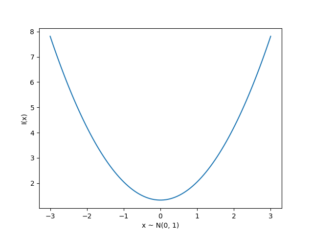
Information theory
Originally developed for message communication, with the intuition that less likely events carry more information, defined for a single event as:
Entropy
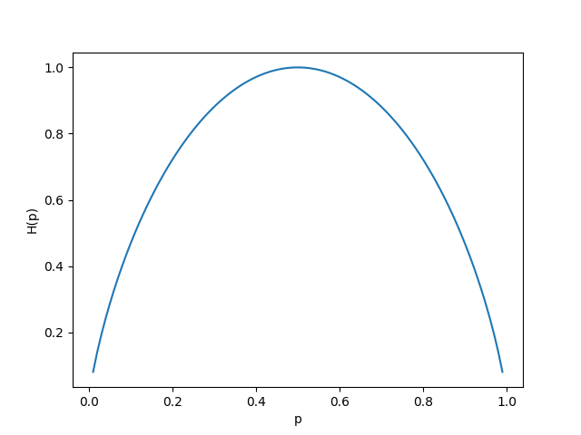
- We can measure the expected information of a distribution as:
- This is called the Shannon entropy
- Measured in bits (base 2) or nats (base )
- :abacus: Find the entropy of a bernoulli distribution
Cross-entropy
- The KL divergence is a measure of the extra information needed to encode a message from a true distribution using an approximate distribution :
- The cross-entropy is a simplification that drops the term :
- Minimizing the cross-entropy is equivalent to minimizing the KL divergence
- If , then and
Cross-entropy loss
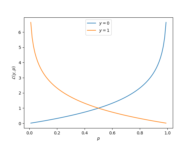
For a true label and predicted , the cross-entropy loss is:
where is the output of the final layer of a neural network (thresholded to obtain the prediction )
This is also called log loss or binary cross-entropy
Terminology for evaluation
-
True positive: predicted positive, label was positive () ✔️
-
True negative: predicted negative, label was negative () ✔️
-
False positive: predicted positive, label was negative () ❌ (type I)
-
False negative: predicted negative, label was positive () ❌ (type II)
-
Accuracy is the fraction of correct predictions, given as:
Precision and recall
-
Precision: Out of all the positive predictions, how many were correct?
-
Recall: Out of all the positive labels, how many were correct?
-
Specificity: Out of all the negative labels, how many were correct?
Confusion matrix
| Predicted Positive | Predicted Negative | |
|---|---|---|
| True Positive | TP | FN |
| True Negative | FP | TN |
- The axes might be reversed, but a good predictor will have strong diagonals
- There’s also the F1 score, or harmonic mean of precision and recall:
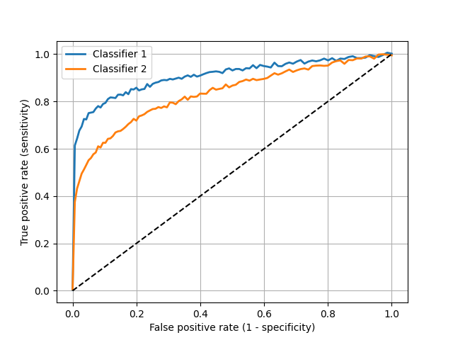
ROC Curves
-
The receiver operating characteristic curve is a plot of the true positive rate (recall or sensitivity) vs. false positive rate (1 - specificity) as the detection threshold changes
-
The diagonal is the same as random guessing
-
A perfect classifier would hug the top left corner
Fun fact: the name comes from WWII radar operators, where true positives were airplanes and false positives were noise
Which classifier is better?
Multiclass case
- For classes, the output is a vector with
- The cross-entropy loss is then:
- For a one-hot encoded vector , this simplifies to: where is the index of the true class
The softmax function
-
For binary classification, the sigmoid function is used to predict the probability of the positive class
-
For multiclass classification, the softmax function is used:
where is the output of neuron in the final layer before the activation function is applied
-
This means that neurons are needed in the final layer, one for each class
Next up: Convolution and NN frameworks
Lecture 6: Modern Neural Networks
Intro to modern neural networks
COMP 4630 | Winter 2024 Charlotte Curtis
Overview
- More decisions when making a neural network
- Weight initialization
- Number of neurons and layers
- Optimization algorithms
- References and suggested reading:
- Scikit-learn book: Chapters 10-11
- Deep Learning Book: Chapter 8
- Understanding Deep Learning: Chapter 7
Revisiting Backpropagation
-
For a network with layers, the gradients of the loss function with respect to the weights in the last layer are given by:
assuming that the output is a function of layer ’s input .
-
At layer , the gradients are computed as:
-
At layer , this becomes:
-
And so on, until we reach the first layer.
-
We are recursively applying the chain rule and re-using the gradients computed at the previous layer
-
This is great for computational efficiency, but it can also lead to vanishing or exploding gradients
Vanishing and Exploding Gradients
- Vanishing/exploding gradients are where the gradients become near zero or near infinity as they are propagated back through the network
- Particularly problematic for recurrent neural networks, where the same weights are multiplied by themselves repeatedly
- Also a problem for very deep networks, and part of the reason that deep learning was not popular until the 2010s
- ❓ What changed?
Consider the variance
- At the input layer, , and has some variance
- Assume and are initialized to 0
- :abacus: What is the variance of ?
- What about after the activation function ?
Initialization strategies
- In 2010, Glorot and Bengio proposed the Xavier initialization for a layer with inputs and outputs:
- Goal is to preserve the variance of the input and output in both directions
- Similar to LeCun initialization, and apparently an overlooked feature of networks from the 1990s
Initialization for ReLU
- Glorot initialization was derived under the assumption of linear activation functions (even though they knew this wasn’t the case)
- In 2015, He et al. proposed the He initialization specifically for ReLU activations:
- The choice of normal vs uniform is apparently not very important
- Default in PyTorch is
Batch normalization
- Also in 2015, Ioffe and Szegedy proposed batch normalization as a way to mitigate vanishing/exploding gradients
- This is simply a normalization at each layer, shifting and scaling the inputs to have a mean of 0 and a variance of 1 (across the batch)
- A moving average of the mean and variance is maintained during training, and used for normalization during inference
- It also ends up acting as regularization, magic!
- ❓ Why wouldn’t you want to use batch normalization?
RELU and its variants
- In early works, the sigmoid or tanh functions were popular
- Both have a small range of non-zero gradients
- ReLU has a stable gradient for positive inputs, but can lead to the dying ReLU problem whereby certain neurons are “turned off”
- ❓ How can we prevent dying ReLUs?
Note: this may not be a problem, and ReLU is cheap. Don’t optimize prematurely unless you’re seeing lots of “dead” neurons.
Number of neurons and layers
- Number of neurons in the input layer is defined by number of features
- Number of neurons in the output layer is defined by prediction task
- In between is a design choice
- Common early choice was a pyramid shape, but it turns out that a stack of layers with the same number of neurons works well too
- Deeper networks can solve more complex problems with the same number of total parameters, but are also prone to vanishing/exploding gradients
Ultimately, yet another a hyperparameter to be tuned
Optimization algorithms: variations on gradient descent
- Gradient descent takes small regular steps, constant or otherwise
- Many variations exist! For example, momentum keeps track of the previously computed gradient and uses it to inform the new step: where is a hyperparameter between 0 and 1
- Adaptive moment estimation (Adam) is a popular choice that adds on an exponentially decaying average of the squared gradients
The Adam optimizer
- Keeps track of first () and second () moments of the gradient, with two exponential decay terms and
- At each time step, the update is now:
- and are typically 0.9 and 0.999, respectively
Regularization via dropout
- Dropout is a regularization technique that randomly sets a fraction of the neurons to zero during training
- During each training pass, a neuron has a probability of being dropped
- Similar to training an ensemble of models then bagging
- Helps to prevent overfitting, but can slow down training
- Typical values: 0.5 for hidden layers, 0.2 for input layers
Choices for starting
From the Deep Learning Book, section 11.2:
- “Depending on the complexity of your problem, you may even want to begin without using deep learning.”
- Tabular data: fully connected, images: convolutional, sequences: recurrent*
- ReLU or variants, with He initialization
- SGD or Adam, add batch normalization if unstable
- Use some kind of regularization, such as dropout
Implementation time
Lecture 7: Convolutional Neural Networks
Convolution and Convolutional Neural Networks
COMP 4630 | Winter 2026 Charlotte Curtis
Overview
- Convolutional neural networks (CNNs) are a type of neural network that is particularly well-suited to image data
- Before we can understand CNNs, we need to understand convolution
- References and suggested reading:
- Scikit-learn book: Chapter 14
- Deep Learning Book: Chapter 9
- 3blue1brown video: What is convolution?
Convolution
-
Convolution is defined as:
-
Or in the discrete case:
-
Can be though of as “flipping” one function and sliding it over the other, multiplying and summing at each point
Example
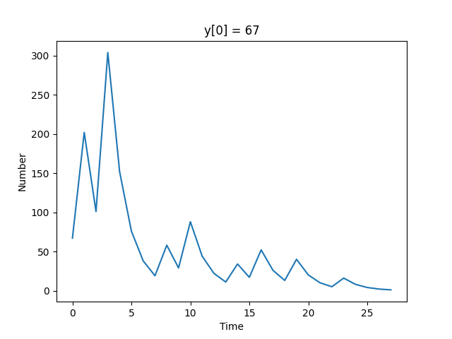
We’re in a hospital dealing with an outbreak. For the first 5 days we have 1 patient on Monday, 2 on Tuesday, etc:
Fortunately, we know how to treat them: 3 doses on day 1, then 2, then 1:
And after 3 days they’re cured.
How many doses do we need on each day?
Convolution in 2D
- Extending to 2D basically adds another summation/integration:
- This can also be extended to higher dimensions
- Caution: a colour image is a 3D array, not a 2D array
- For typical image processing applications, the colour channels are convolved independently such that the output is still a 3D array
Convolution kernels
- Typically there is a small kernel that is convolved with the input
- This is just the smaller of the two functions in the convolution
- ❓ What happens at the edges of the input?

Some common kernels
- Averaging:
- Differentiation:
- Sizes are commonly chosen to be 3x3, 5x5, 7x7, etc.
- ❓ Why divide by 9?
- ❓ Why odd sizes?
- ❓ What effect do you think these kernels will have on an image?
A side tangent on frequency representation
- Any signal can be represented as a weighted summation of sinusoids
- For a discrete signal , you can think of this as:
- Or, using Euler’s formula : where the complex coefficients
Fourier Transform
- To figure out what the coefficients are, we can use the Discrete Fourier Transform (DFT): where each element of is the coefficient for frequency
- The Fast Fourier Transform (FFT) computes the DFT in time
- Convolution is
Convolution is multiplication in frequency
- Sometimes it is useful to use the Fourier Transform to obtain a frequency representation of an image (or signal)
- In the frequency domain, convolution is simply element-wise multiplication
- This allows for some efficient operations such as blurring/sharpening an image, as well as some fancy stuff like deconvolution
- Sharp edges in space become ringing in frequency, and vice versa
- ❓ why do CNNs operate in the spatial domain?
Convolutional neural networks
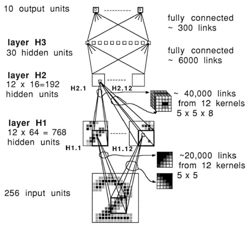
- 1958: Hubel and Wiesel experiment on cats and reveal the structure of the visual cortex
- Determine that specific neurons react to specific features and receptive fields
- Modelled in the “neocognitron” by Kunihiko Fukushima in 1980
- LeCun’s work in the 1990s led to modern CNNs
Why CNNs?
- A fully connected network has a 1:1 mapping of weights to inputs
- Fine for MNIST (28x28) pixels, but quickly grows out of control
- ❓ If you train a (fully connected) network on 100x100 images, how would you infer on 200x200 images?
- ❓ What if an object is shifted, rotated, or flipped within the image?

Convolutional layers
- A convolution layer is a set of kernels whose weights are learned
- Instead of the straight up weighted sum of inputs, the input image is convolved with the learned kernel(s)
- The output is often referred to as a feature map
- The dimensionality of the feature map is determined by the:
- Size of the input image
- Number of kernels
- Padding (usually “same” or “valid”)
- “Stride”, or shift of the kernel at each step
Dimensionality examples
| Input | Kernel | Stride | Padding | Output |
|---|---|---|---|---|
| 1 | same | |||
| 2 | same | |||
| 1 | valid | ??? |
- The number of channels has no impact on the depth of the output: the number of kernels determines the depth of the output
- The colour channels are convolved independently, then summed
Number of parameters example
- Input:
- Kernel:
- Bias terms: 32
- Total parameters:
While convolution only happens in 2D, the kernel can be thought of as a 3D volume - there’s a separate trainable kernel for each channel
Pooling layers
Pooling layers are used to reduce the dimensionality of the feature maps (aka downsampling) by taking the maximum or average of a region
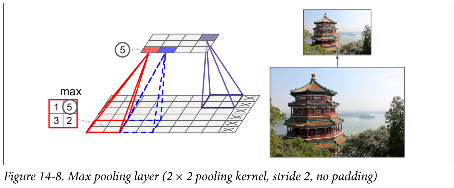
- ❓ Why would we want to downsample?
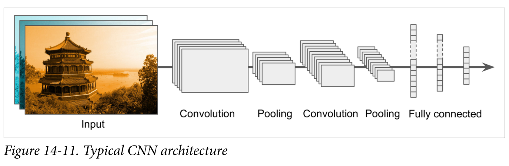
Putting it all together
Backpropagating CNNs
- After backpropagating through the fully connected head, we need to backpropagate through the:
- Pooling layer
- Convolution layer
- The pooling layer has no learnable parameters, but it needs to remember which input was maximum (all the rest get a gradient of 0)
- The convolution layer is trickier math, but it ends up needing another convolution - this time with the kernel transposed
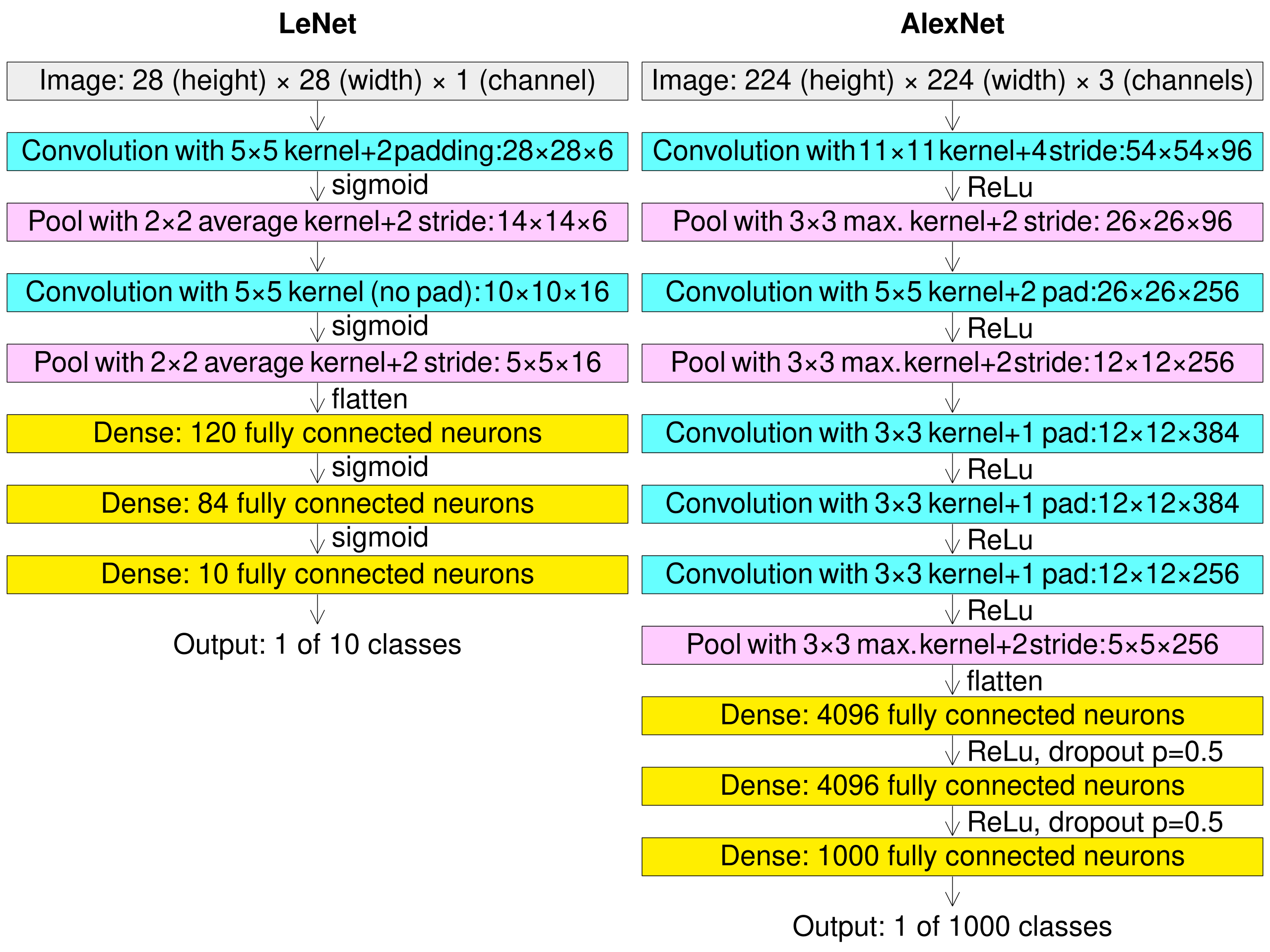
LeNet (1998) vs AlexNet (2012)
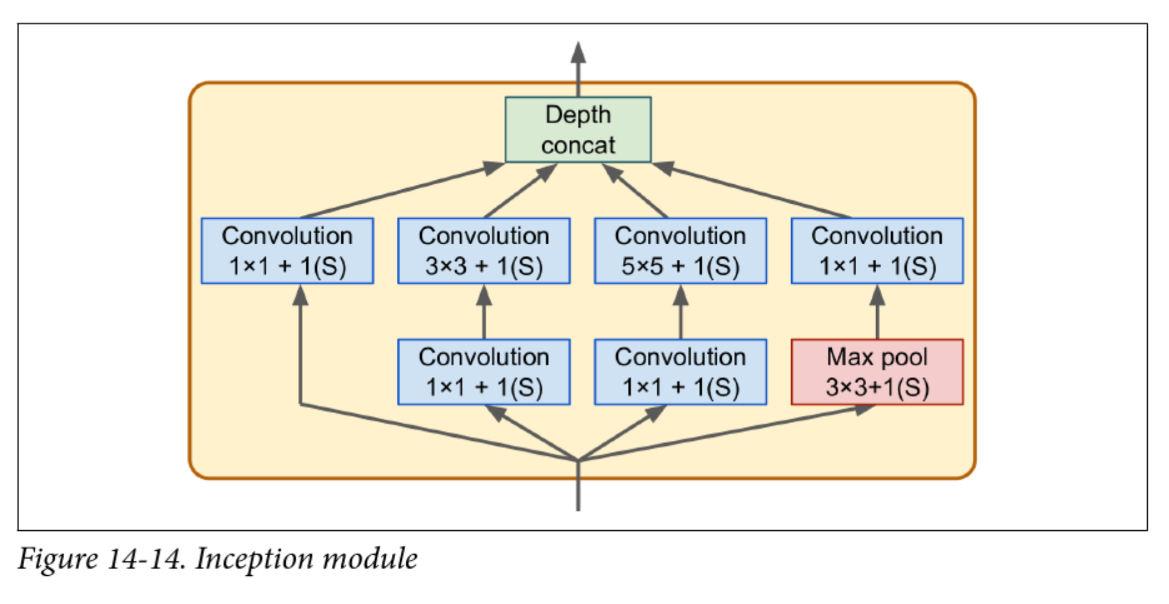
Inception v1 aka GoogLeNet (2014)
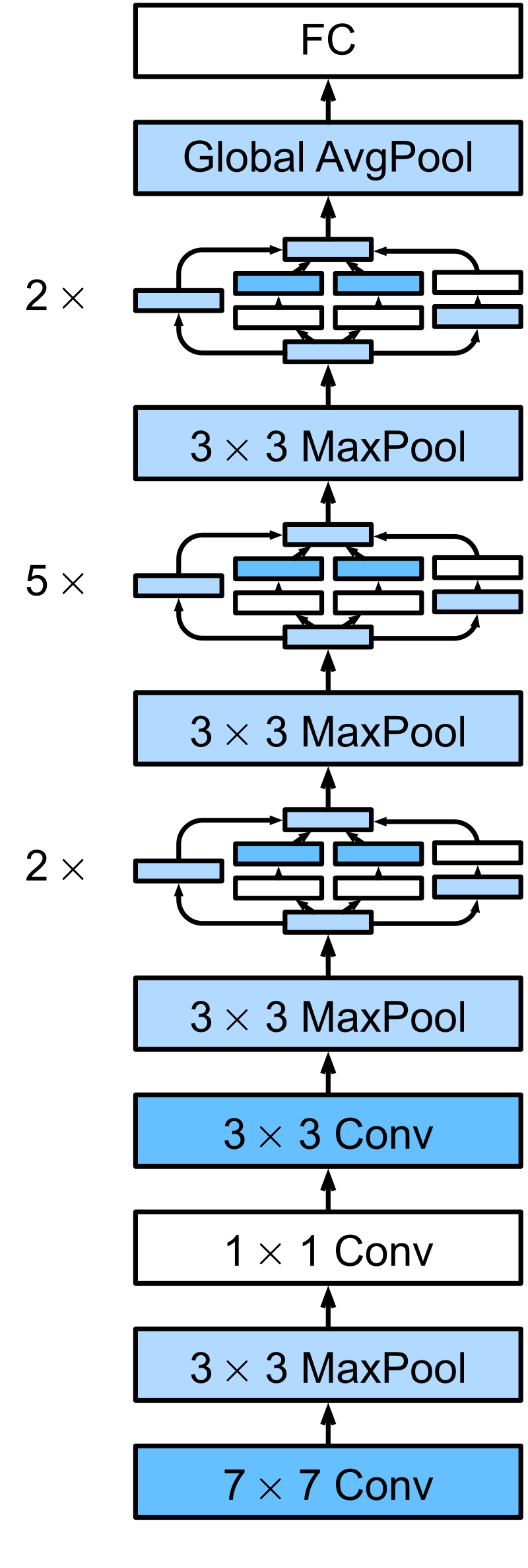
- Struggled with vanishing gradients
- v2 introduced batch normalization
VGG (2014)
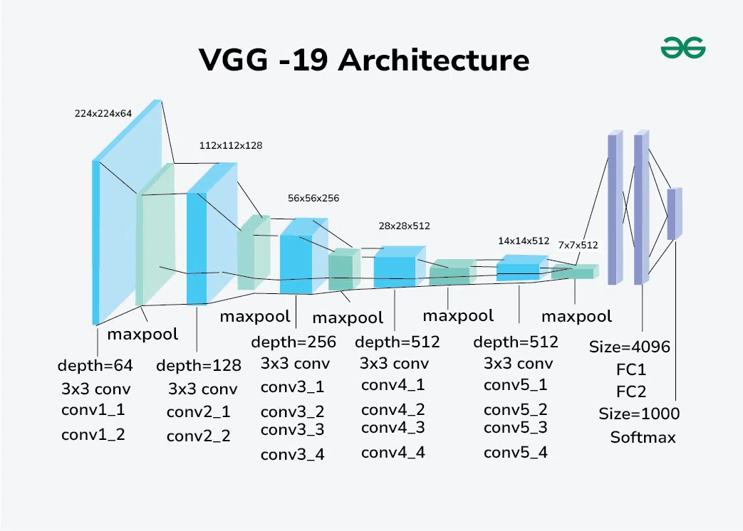
- Simple architecture, but “very” deep (16 or 19 layers)
- Fixed the convolution hyperparameters and focused on depth
ResNet (2015)
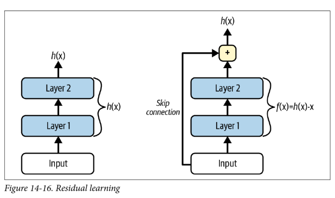
- Key innovation: easier to learn “identity” functions ()
- If a layer outputs 0, it doesn’t kill the gradient
- Even deeper, e.g. ResNet-152
Transfer Learning
“If I have seen further, it is by standing on the shoulder of giants” – Isaac Newton
- Transfer learning copy pastes a trained network into a new task
- You can select which layers to keep, which to freeze, and which to re-train
- You can also drop new layers on top of the old ones
- Most of the time you want to freeze the early layers and add a new “head”
Data Augmentation
-
Garbage in, garbage out
-
We can artificially increase diversity with data augmentation:
- Random crops, flips, rotations
- Rescaling/resizing
- Changing colours
-
AutoAugment does a bunch of this automatically
Next up: RNNs
Lecture 8: Recurrent Neural Networks
Recurrent Neural Networks
COMP 4630 | Winter 2026 Charlotte Curtis
Overview
- Dealing with sequence data
- Feedforward vs recurrent networks
- References and suggested reading:
- Scikit-learn book: Chapter 15
- Deep Learning Book: Chapter 10
Sequence data
- So far we’ve been talking about images, tabular data, and other “static” data
- ❓ What are some examples of sequence data?
Non-RNN Approaches
As usual, you don’t always need a deep learning solution :hammer:
- ❓ What is an example of a “naive” approach?
- ❓ What are some limitations of naive approaches?
Autoregressive Moving Average
- Models to predict time series with a weighted average of past value where
- Key assumption: data is stationary (mean and variance don’t change)
- ARIMA adds on “integration” or “differencing” to account for trends
ARIMA
- Autoregressive parameter : How many steps back to average?
- Moving average parameter : How many previous errors to average?
- Integrative parameter : How many “differencing” rounds to perform before applying ARMA?
can be thought of as approximating the order polynomial
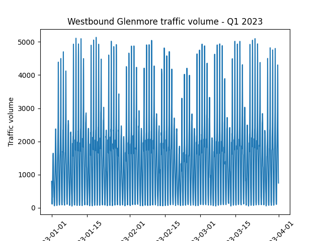
Trends, Seasonality, and Assumptions
- ❓ Are there any obvious trends in the data?
- ❓ What about non-obvious trends?
- ❓ How might this dataset be treated differently from the previous one?
Feedforward vs recurrent networks
- Feedforward: data flows in one direction (then backpropagated)
- Recurrent: data can flow in loops
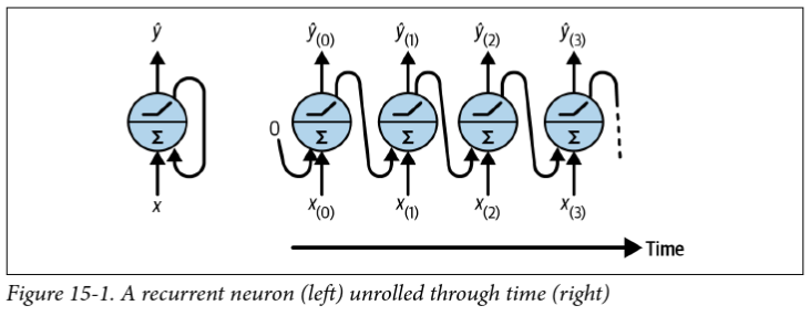
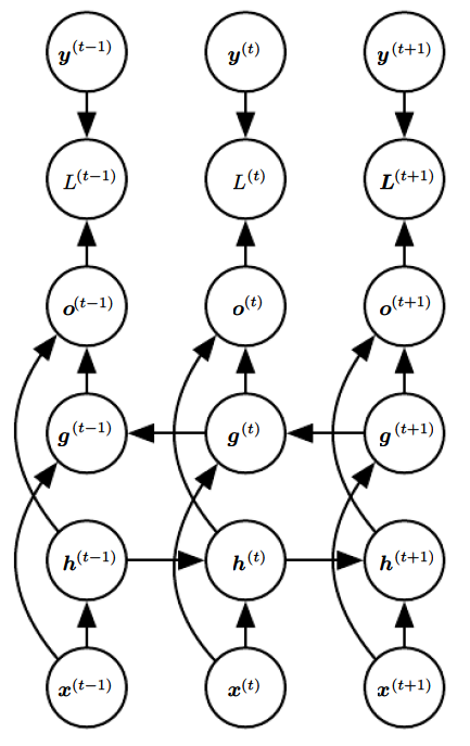
Recurrent layers
- The simplest recurrent layer has a single feedback connection where is the activation function and and are weight matrices
- “Backpropagation through time” (BPTT) is exactly the same as regular backpropagation through the unrolled network
- ❓ What kind of issues might arise during training?
- ❓ What are some limitations of this approach?
- ❓ How can we deal with for ?
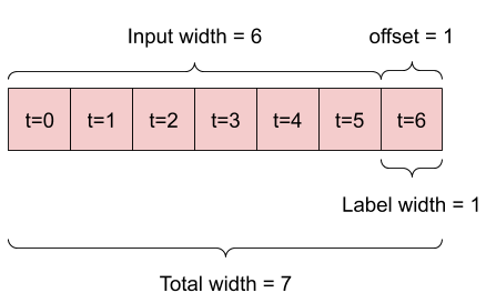
Preparing data for RNNs
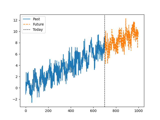
- The data format depends on the task, e.g. do you want to predict:
- The next value in a sequence (e.g. predictive text)
- The next values in a sequence (e.g. stock prices)
- The next sequence in a set of sequences (e.g. language translation)
- Let’s start with predicting the next value in a sequence
Activation Functions for RNNs
- The default activation function in tensorflow/PyTorch is
tanh - ❓ What is different about RNNs that might influence the choice of activation function?
- ❓ How might we normalize sequence data?
Beyond the “next value”
- Option 1: Use the single-prediction RNN repeatedly
- Option 2: Train the RNN to predict multiple values at once
- Easy change model-wise, but data preparation is trickier
ninputs,noutputs
- Option 3: Use a “sequence to sequence” model
- Even trickier data preparation, but
ninputs are predicted at each time step instead of just at the end
- Even trickier data preparation, but
Seq2seq input/target examples
| Input | Target | |
|---|---|---|
| 1 | [0, 1, 2] | [1, 2, 3] |
| 2 | [0, 1, 2] | [[1, 2], [2, 3], [3, 4]] |
| 3 | [0, 1, 2] | [[1, 2, 3], [2, 3, 4], [3, 4, 5]] |
Problems with long sequences
- Gradient vanishing/exploding
- Choose activation functions and initialization carefully
- Consider “Layer normalization” (across features)
- “Forgetting” early data
- Skip connections through time
- “Leaky” RNNs
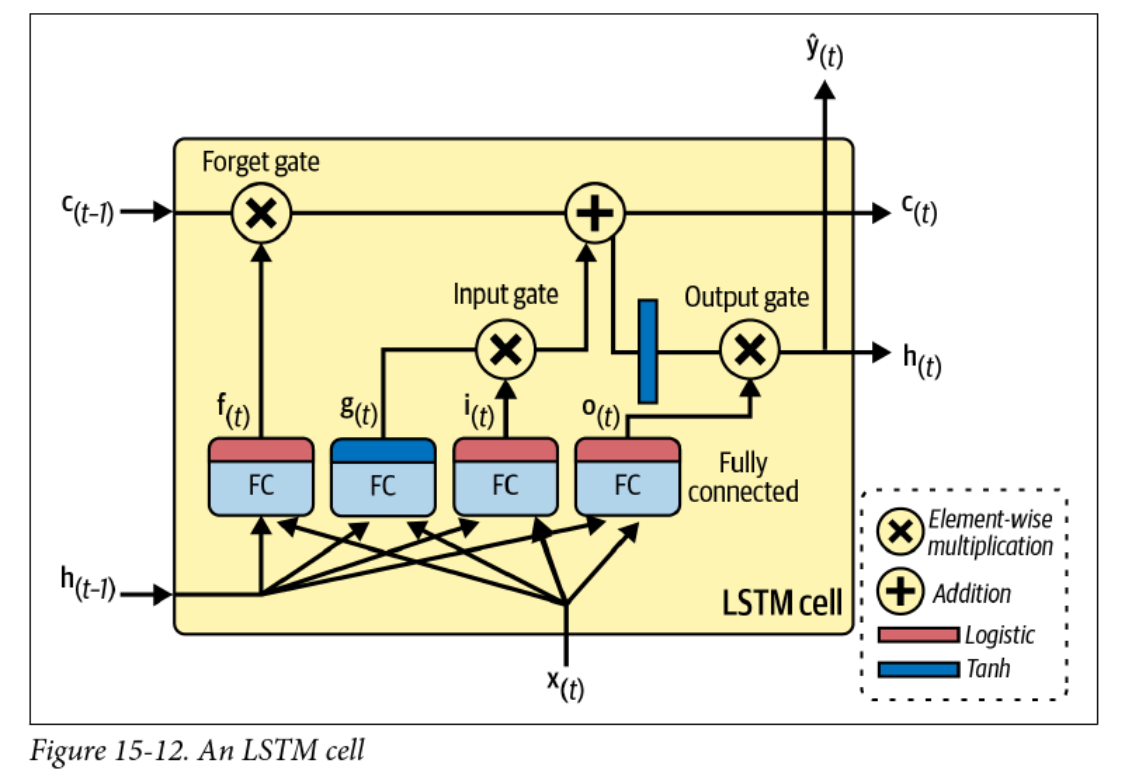
- Long short-term memory (LSTM)
- Computational efficiency and memory constraints
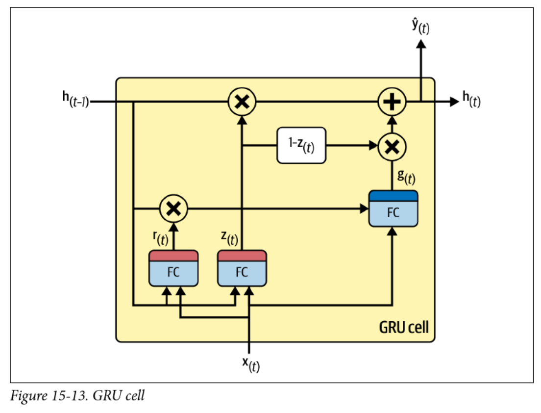
- Gated recurrent units (GRUs)
Skip connections and leaky RNNs
- Simple way of preserving earlier data:
- Vanilla RNN: depends on only
- Skip connection: depends on , , , etc.
- Leaky RNN has a smooth “self-connection” to dampen the exponential:
- Not common approaches anymore, as LSTM, GRU, and especially attention mechanisms are more popular
Long Short-Term Memory (LSTM)
Gated Recurrent Units (GRUs)
Next up: Natural Language Processing
Preview: Natural Language Processing
- Natural Language Processing (NLP) is a field of study that focuses on the interaction between computers and human language.
- RNNs are widely used in NLP tasks such as language modeling, machine translation, sentiment analysis, and text generation.
- Language modeling involves predicting the next word in a sequence of words, which can be done using RNNs.
- Machine translation uses RNNs to translate text from one language to another.
- Sentiment analysis aims to determine the sentiment or emotion expressed in a piece of text, and RNNs can be used for this task.
- Text generation involves generating new text based on a given input, and RNNs are commonly used for this purpose.
Preview: Natural Language Processing
- What is Natural Language Processing (NLP)?
- Common NLP tasks:
- Language modeling
- Machine translation
- Sentiment analysis
- Text generation
- How RNNs are applied in NLP
Preview: Natural Language Processing
- NLP in 2026 is dominated by large language models (LLMs) like GPT-4o, Claude, and Gemini
- Transformer-based architectures have largely replaced RNNs for most NLP tasks
- Key capabilities of modern NLP systems:
- Multi-modal understanding (text, images, audio, video)
- Long-context reasoning (millions of tokens)
- Agentic behaviour: tool use, planning, and self-correction
- ❓ If transformers have replaced RNNs, why are we still studying them?
Lecture 9: Natural Language Processing
Natural Language Processing
COMP 4630 | Winter 2026 Charlotte Curtis
Overview
- Text to tokens
- Tokens to embeddings
- Embeddings to predictions
- References and suggested reading:
- Scikit-learn book: Chapter 16
- Deep Learning Book: Chapter 12
Tokenization
-
Consider the sentence:
“The cat sat on the mat.”
-
This can be split up into individual words or tokens:
[“The”, “cat”, “sat”, “on”, “the”, “mat”, “.”]
-
❓ what other ways could we tokenize this sentence?
-
❓ what about punctuation, capitalization, etc.?
RNN + tokens: predict the next character
- Just like predicting the next day’s weather or stock price, we can predict the next character in a sentence using an RNN
- Input tokens:
['T', 'h', 'e', ' ', 'c', 'a', 't', ' ', 's', 'a', 't', ' ', 'o', 'n', ' ', 't', 'h', 'e', ' ', 'm', 'a', 't', '.'] - Numeric representation:
[20, 8, 5, 0, 3, 1, 20, 0, 19, 1, 20, 0, 15, 14, 0, 20, 8, 5, 0, 13, 1, 20, 2] - We could train an RNN model to predict the next character
- For more info check out Andrej Karpathy’s blog post, one of the sources for the Scikit-learn chapter
Repeatedly predicting the next character
- To predict whole sentences from a starting point, we can predict the next character and append it to the input, then predict again
- In practice this tends to get stuck in loops:
Input:
"to be or not"Output:"to be or not to be or not to be or not..." - ❓ how might we avoid this?
- ❓ could we just predict the next whole word instead?
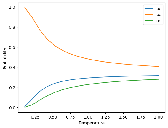
Controlled chaos: softmax temperature
- The softmax is defined as: where is a vector of logits, or log probabilities
- This estimates the probability of class out of classes
- Adding a temperature parameter :
Temperature Example
- Vocab =
["to", "be", "or"] - Assume that the “logits”
- Sample the next word from the resulting distribution
In the beginning, there were -grams
-
A simple way to represent text is as a bag of -grams
-
unigram: single words (aka “Bag of Words”):
[“the”, “cat”, “sat”, “on”, “the”, “mat”]
-
bigram: pairs of words:
[“the cat”, “cat sat”, “sat on”, “on the”, “the mat”]
-
trigram: triples of words:
[“the cat sat”, “cat sat on”, “sat on the”, “on the mat”]
Predictive text with -grams
-
Given a sequence of tokens, we can predict the probability of the th token given the previous tokens:
-
Each of these conditional probabilities can be estimated from the frequency of the -grams in a corpus
-
The most likely next word is the one with the highest probability
-
❓ What are some limitations of this approach?
-grams challenges
- -grams lose the meaning of words:
- “The cat sat on the mat”
- “The dog sat on the rug”
- Also subject to the curse of dimensionality
- Vocabulary with size leads to possible -grams
- Most -grams will not be present in the corpus!
- ❓ Can you think of an -gram modification that could help this problem?
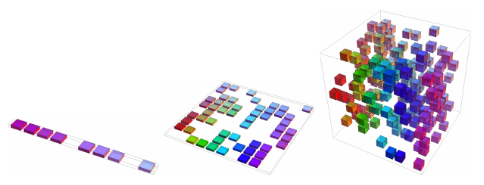
Side note: The curse of dimensionality
- Data is often represented as samples with features each
- As increases, the number of samples required to cover the space increases exponentially
- Also called problem
Word embeddings
-
Alternative solution: represent individual words as vectors, or embeddings
-
❓ How are these embeddings defined?
Word Embedding cat [0.2, 0.3, 0.5]dog [0.1, 0.4, 0.4]mat [0.5, 0.2, 0.2]rug [0.4, 0.1, 0.1]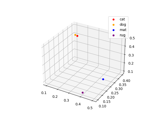
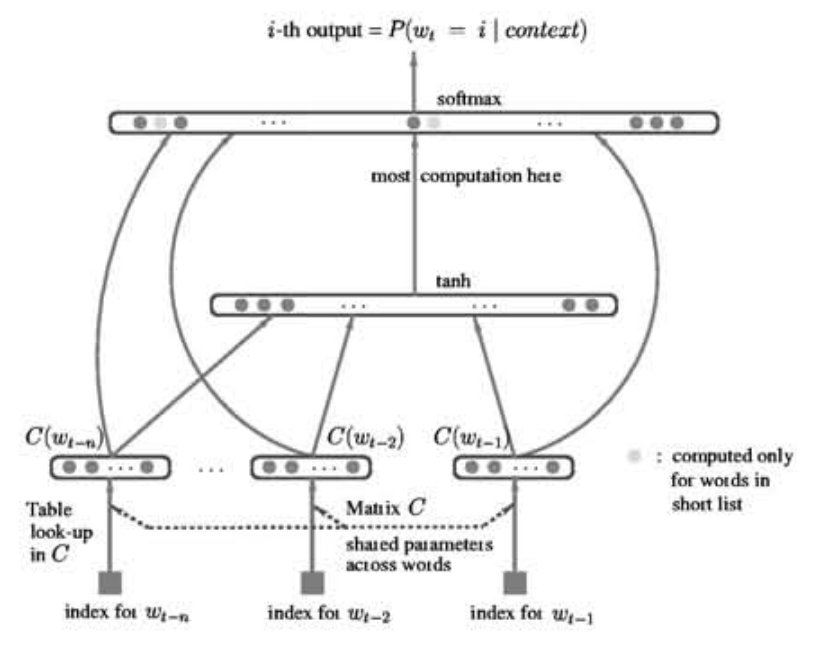
Learning word embeddings
- Wednesday we’ll discuss the influential Word2Vec paper, but it wasn’t the first time embeddings were learned as part of a network
- The concept was first presented successfully by Bengio in 2001
So we have embeddings, now what?
- We can use these embeddings as input to a neural network
- Applications:
- Sentiment analysis: is a review/tweet/comment positive or negative?
- Named entity recognition: who/what is mentioned in a text?
- Machine translation: convert text from one language to another
- Predictive text: what word comes next?
- Text generation: create new text based on a given input
Sentiment analysis
General process:
- Standardize and tokenize the text
- Add an embedding layer (trainable or pre-trained)
- Add a recurrent layer, such as a GRU
- Add a dense layer with sigmoid activation
To Colab!
This is the process you’ll be following for Assignment 3
Sequence to Sequence models
Back to RNNs
-
RNNs predict the future based on the past
-
This is exactly what we want for predicting stock prices, weather, etc
-
❓ What about translating a sentence from one language to another?
Time flies like an arrow; fruit flies like a banana.
-
❓ Can you think of a way to get RNNs to see the future?
Bidirectional RNNs
-
Simple approach: just reverse the sequence
Pretraining
- Embeddings like Word2Vec have been trained on large corpora
- Surely this provides a great starting point for our models!
- ❓ what are some potential drawbacks?
- ELMo was introduced in 2018 specifically to address the limitations of Word2Vec and GloVe (another popular embedding)
“Our representations differ from traditional word type embeddings in that each token is assigned a representation that is a function of the entire input sentence. We use vectors derived from a bidirectional LSTM that is trained with a coupled language model objective on a large text corpus” – Peters et al
Subword Tokenization
- Word embeddings are great, but still have limitations
- ELMo uses character tokenization to handle out-of-vocabulary words
- In between characters and words are subwords
"This warm weather is enjoyable""This", "warm", "weath", "er", "is", "enjoy", "able"
- Byte Pair Encoding is the most common subword tokenization method, used by GPT and BERT
- ❓ What are some advantages of subword tokenization?
Machine Translation
| English | Spanish |
|---|---|
| My mother did nothing but weep | Mi madre no hizo nada sino llorar |
| Croatia is in the southeastern part of Europe | Croacia está en el sudeste de Europa |
| I would prefer an honorable death | Preferiría una muerte honorable |
| I have never eaten a mango before | Nunca he comido un mango |
- ❓ What kind of challenges can you think of?
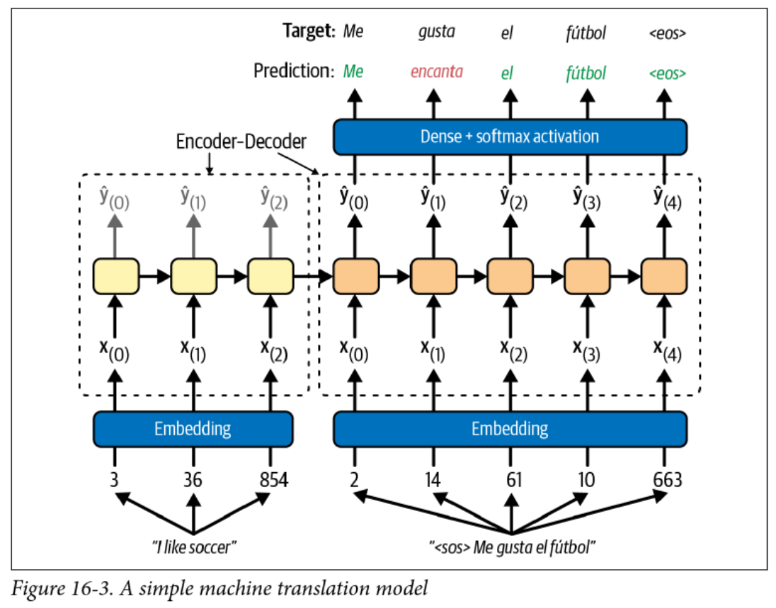
Encoder-Decoder Models
- RNNs can convert an arbitrary length sequence into a fixed length vector
- RNNs can convert a fixed length vector into an arbitrary length sequence
- Why not use two RNNs to convert a sequence to a sequence?
- The output head is a softmax layer with one node for each word in the target vocabulary
Teacher Forcing
- This model uses teacher forcing to train the decoder
- It feels like cheating, but this involves feeding the correct output to the decoder at each time step
- This speeds up training and can improve performance
- Avoids the whole backpropagation through time thing and makes training of RNNs parallelizable
- ❓ What are the implications at inference time?
Coming up next: Attention mechanisms and Transformers
Lecture 10: Transformers
Transformers and Large Language Models
COMP 4630 | Winter 2026 Charlotte Curtis
Overview
- Attention mechanisms
- Transformers and large language models
- Multi-head attention, positional encoding, and magic
- BERT, GPT, Llama, etc.
- References and suggested readings:
- Scikit-learn book: Chapter 16
- d2l.ai: Chapter 11
Attention Overview
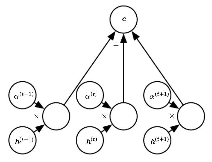
- Basically a weighted average of the encoder states, called the context
- Weights usually come from a softmax layer
- ❓ what does the use of softmax tell us about the weights?
Encoder-Decoder with Attention
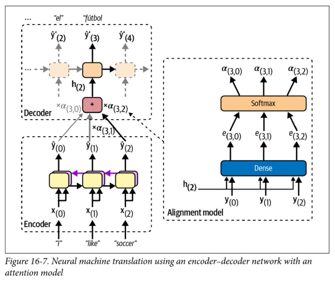
- The alignment model is used to calculate attention weights
- The context vector changes at each time step!
Attention Example
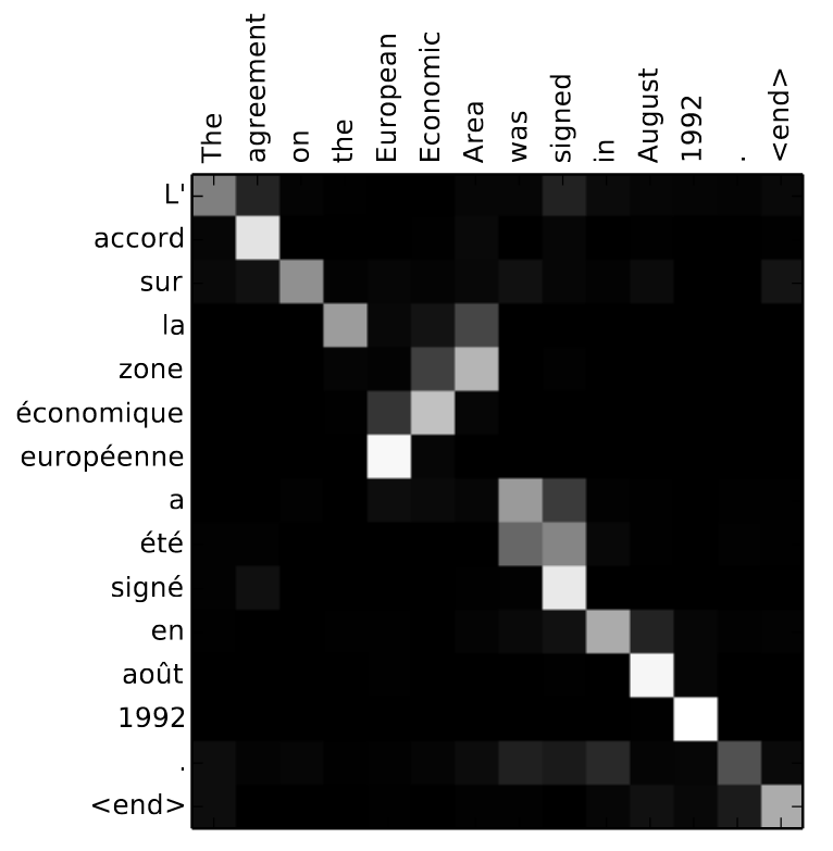
- Attention weights can be visualized as a heatmap
- ❓ What can you infer from this heatmap?
The math version
The context vector at each step is computed from the alignment weights as:
where is the encoder output at step and is computed as:
where is the alignment score or energy between the decoder hidden state at step and the encoder output at step .
Different kinds of attention
- The original Bahdanau attention (2014) model: where , , and are learned parameters
- Luong attention (2015), where the encoder outputs are multiplied by the decoder hidden state (dot product) at the current step
- ❓ What might be a benefit of dot-product attention?
Attention is all you need
- Some Googlers wanted to ditch RNNs
- If they can eliminate the sequential nature of the model, they can parallelize training on their massive GPU (TPU) clusters
- Problem: context matters!
- ❓ How can we preserve order, but also parallelize training?
Transformers
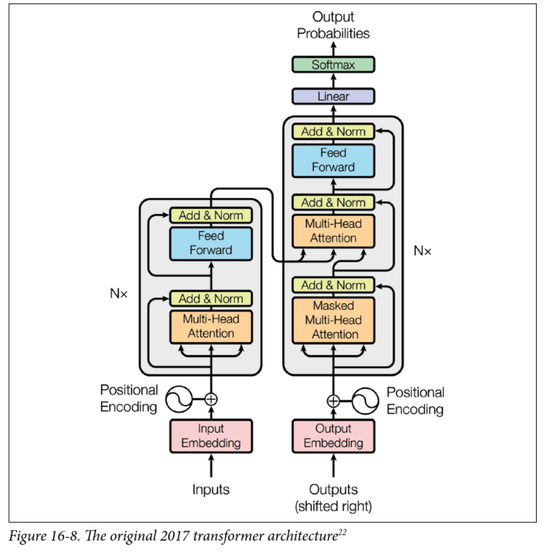
- Still encoder-decoder and sequence-to-sequence
- encoder/decoder layers
- New stuff:
- Multi-head attention
- Positional encoding
- Skip (residual) connections and layer normalization
Multi-head attention
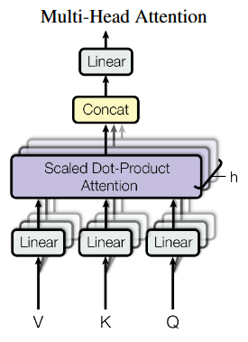
- Each input is linearly projected times with different learned projections
- The projections are aligned with independent attention mechanisms
- Outputs are concatenated and linearly projected back to the original dimension
- Concept: each layer can learn different relationships between tokens
What are V, K, and Q?
- Attention is described as querying a set of key-value pairs
- Kind of like a fuzzy dictionary lookup
- is an matrix, where is the dimension of the keys
- is an matrix
- is an matrix
- The product is , representing the alignment score between queries and keys (dot product attention)
The various (multi) attention heads
- Encoder self-attention (query, key, value are all from the same sequence)
- Learns relationships between input tokens (e.g. English words)
- Decoder masked self-attention:
- Like the encoder, but only looks at previously generated tokens
- Prevents the decoder from “cheating” by looking at future tokens
- Decoder cross-attention:
- Decodes the output sequence by “attending” to the input sequence
- Queries come from the previous decoder layer, keys and values come from the encoder (like prior work)
Positional encoding
- By getting rid of RNNs, we’re down to a bag of words
- Positional encoding re-introduces the concept of order
- Simple approach for word position and dimension :
- resulting vector is added to the input embeddings
- ❓ Why sinusoids? What other approaches might work?
Other positional encodings
- Appendix D of the new version of Hands-on Machine Learning goes into detail about positional encodings, particularly for very long sequences
- Sinusoidal encoding is no longer used in favour of relative approaches
- Introduces locality bias
- Removes early-token bias
- Example: learnable bias for position in , clamped to a max
- Only bias terms to learn, regardless of sequence length
Interpretability
- The arXiv version of the paper has some fun visualizations
- This is Figure 5, showing learned attention from two different heads of the encoder self-attention layer
A smattering of Large language models
- GPT (2018): Train to predict the next word on a lot of text, then fine-tune
- Used only masked self-attention layers (the decoder part)
- BERT (2018): Bidirectional Encoder Representations from Transformers
- Train to predict missing words in a sentence, then fine-tune
- Used unmasked self-attention layers only (the encoder part)
- GPT-2 (2019): Bigger, better, and capable even without fine-tuning
- Llama (2023): Accessible and open source language model
- DeepSeek (2024): Significantly more efficient, but accused of being a distillation of OpenAI’s models
Hugging Face
-
Hugging Face provides a whole ecosystem for working with transformers
-
Easiest way is with the
pipelineinterface for inference:from transformers import pipeline nlp = pipeline("sentiment-analysis") # for example nlp("Cats are fickle creatures") -
Hugging Face models can also be fine-tuned on your own data
And now for something completely different: Deep reinforcement learning
Lecture 11: Reinforcement Learning
(Deep) Reinforcement Learning
COMP 4630 | Winter 2026 Charlotte Curtis
Overview
- Terminology and fundamentals
- Q-learning
- Deep Q Networks
- References and suggested reading:
- Scikit-learn book: Chapter 18
- d2l.ai: Chapter 17
Reinforcement Learning + LLMs
Terminology
- Agent: the learner or decision maker
- Environment: the world the agent interacts with
- State: the current situation
- Reward: feedback from the environment
- Action: what the agent can do
- Policy: the strategy the agent uses to make decisions
Classic example: Cartpole
The Credit Assignment Problem
- Problem: If we’ve taken 100 actions and received a reward, which ones were “good” actions contributing to the reward?
- Solution: Evaluate an action based on the sum of all future rewards
- Apply a discount factor to future rewards, reducing their influence
- Common choice in the range of to
- Example of actions/rewards:
- Action: Right, Reward: 10
- Action: Right, Reward: 0
- Action: Right, Reward: -50
Policy Gradient Approach
- If we can calculate the gradient of the expected reward with respect to the policy parameters, we can use gradient descent to find the best policy
- Loss function example: REINFORCE (Williams, 1992)
where:
- = output probability for action given state
- = reward at timestep
- = model parameters
Value-based methods
- Policy gradient approach is direct, but only really works for simple policies
- Value-based methods instead explore the space and learn the value associated with a given action
- Based on Markov Decision Processes (review from AI?)
Markov Chains
- A Markov Chain is a model of random states where the future state depends only on the current state (a memoryless process)
- Used to model real-world processes, e.g. Google’s PageRank algorithm
- ❓ Which of these is the terminal state?
Markov Decision Processes
- Like a Markov Chain, but with actions and rewards
- Bellman optimality equation:
Iterative solution to Bellman’s equation
Value Iteration:
- Initialize for all states
- Update using the Bellman equation
- Repeat until convergence
Problem: we still don’t know the optimal policy
Q-Values
Bellman’s equation for Q-values (optimal state-action pairs):
Optimal policy :
For small spaces, we can use dynamic programming to iteratively solve for
Q-Learning
- Q-Learning is a variation on Q-value iteration that learns the transition probabilities and rewards from experience
- An agent interacts with the environment and keeps track of the estimated Q-values for each state-action pair
- It’s also a type of temporal difference learning (TD learning), which is kind of similar to stochastic gradient descent
- Interestingly, Q-learning is “off-policy” because it learns the optimal policy while following a different one (in this case, totally random exploration)
Q-Learning Update rule
-
At each iteration, the Q estimate is updated according to:
-
Where:
- is the estimated value of taking action in state
- is the learning rate (decreasing over time)
- is the immediate reward
- is the discount factor
- is the maximum Q-value for the next state
Exploration policies
- ❓ How do you balance short-term rewards, long-term rewards, and exploration?
- Our small example used a purely random policy
- -greedy chooses to explore randomly with probability , and greedily with probability
- Common to start with high and gradually reduce (e.g. 1 down to 0.05)
Challenges with Q-Learning
- ❓ We just converged on a 3-state problem in 10k iterations. How many states are in something like an Atari game?
- ❓ How do we handle continuous state spaces?
One approach: Approximate Q-learning:
- approximates the Q-value for any state-action pair
- The number of parameters can be kept manageable
- Turns out that neural networks are great for this!
Deep Q-Networks
- We know states, actions, and observed rewards
- We need to estimate the Q-values for each state-action pair
- Target Q-values:
- is the observed reward, is the next state
- is the network’s estimate of the future reward
- Loss function:
- Standard MSE, backpropagation, etc.
Challenges with DQNs
- Catastrophic forgetting: just when it seems to converge, the network forgets what it learned about old states and comes crashing down
- The learning environment keeps changing, which isn’t great for gradient descent
- The loss value isn’t a good indicator of performance, particularly since we’re estimating both the target and the Q-values
- Ultimately, reinforcement learning is inherently unstable!
The last topic: Geneterative AI and ethics


GenAI + Ethics Discussion
- Generative images have gotten really good
- What can we do? What should we do?
Lecture 12: Ethics Discussion
Generative AI, ethics, and policies
COMP 4630 | Winter 2026 Charlotte Curtis
Guiding questions for discussion
- What are some ways that AI can be helpful? Harmful?
- What are some ways that AI is used?
- Axes: intent (malicious <-> innocent), impact (harmful <-> helpful)
- What concerns do you have about AI in general?
- What about in education, specifically at MRU?
- What would you like to see in an AI policy at MRU?
Case study: vibe coding
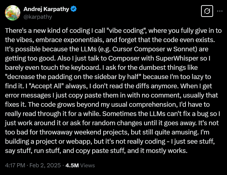
Costs* of:
- Voice to text
- Code generation
- Debugging
- at ~3 Wh/request
April fools?
- Yesterday (March 31st, 2026), Claude Code’s source code was accidentally leaked
- It’s an interesting code base to browse through, notably:
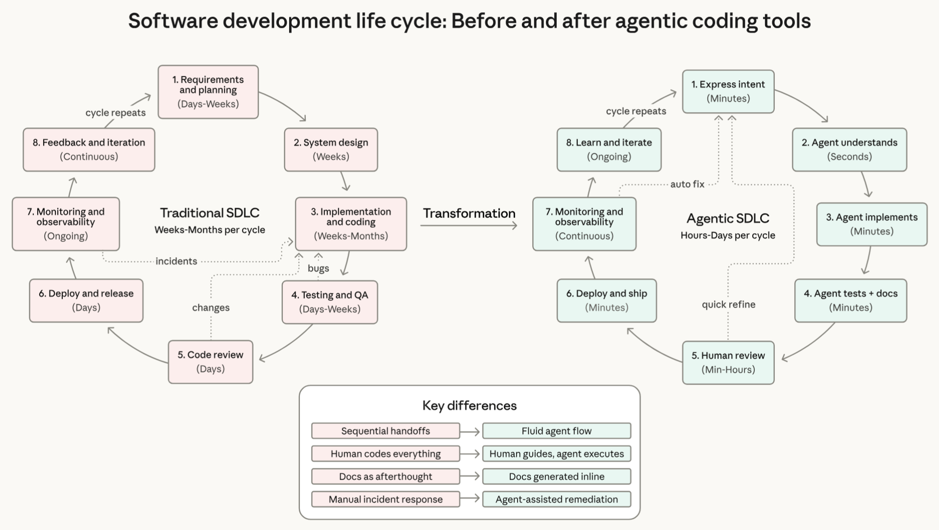
Impact
- How do you, as CS majors, feel about these trends?
- Have you tried using agentic coding tools?
- What is the true cost of agentic coding?
- A recent paper attempts to quantify token usage by task
- Environmental impact, energy consumption, financial cost
Coming up next
- Easter break, no class on Monday
- Wednesday: One last journal club presentation (YOLO) and a smattering of additional topics (autoencoders, object detection, image generation?)
- Monday: last day of class! Assignment 3 results, project checkpoint discussions. Maybe some kind of treats.
Tutorial 1: Data exploration and wrangling
Before building a machine learning model, it is important to understand and wrangle your data into an appropriate numeric format. In this tutorial, we’ll look at how I like to set up my projects and some tips for exploratory visualizations.
Part 1: Project configuration
Tutorials are not marked in this course, so it’s up to you to keep track of them separately. I recommend copying the this directory to a new location rather than forking the entire w26 repo and working out of that, otherwise you’ll have a bunch of merge conflicts and extra stuff if you want to submit a PR to the main repo. Alternatively, you can create a fork and work within a separate branch.
Tools:
Part 2: Exploratory visualizations
Visualizations for the purposes of exploring data (rather than communicating results) can be “quick and dirty”, but there are some guidelines to consider, as well as a few tricks that can help.
Follow along with the notebook and answer the various TODOs.
Part 3: Reverse engineer a cleaned dataset
- Create a new .ipynb file to explore this new dataset
- Read the raw data into a pandas DataFrame. You can either download the zip file, or install the
ucimlrepopackage and fetch the data directly. - Read the pre-processed version into a different pandas DataFrame.
- Try to answer the following questions:
- How were the categorical features handled?
- Were any of the numerical categories manipulated?
- What additional transformations might be useful for this dataset?
Tutorial 2: Linear algebra and NumPy exercises
Linear algebra is foundational to machine learning, and NumPy is a mature Python library that allows you to work efficiently with matrices and vectors.
For this tutorial, I’ll be providing a printed worksheet with some exercises to do by hand. You can then check your answers using NumPy. This serves to both refresh your memory on linear algebra as well as gain some familiarity working with NumPy.
NumPy Basics
By convention, NumPy is imported with the name np:
import numpy as np
You can then create an N-dimensional array by passing a standard Python list to np.array:
v = np.array([1, 2]) # a 1-D vector
print(v.shape) # prints (2, )
A = np.array([[1, 2], [3, 4]]) # a 2-D matrix
print(A.shape) # prints (2, 2)
The default multiplication operator is element-wise. If you want to use matrix multiplication, use the @ operator, or dot function for vectors:
print(A * v)
print(A @ v)
print(v.dot(v)) # or np.dot(v, v)
Output:
[[1 4]
 [3 8]]

[5, 11]

5
Transposing a matrix is quite simple, but the inverse needs the linalg submodule:
print(A.T) # Transpose
print(np.linalg.inv(A)) # Matrix inverse
Output:
[[1 3]
 [2 4]]

[[-2.   1. ]
 [ 1.5 -0.5]]
Similarly, linalg has useful functions like norm, det, solve… getting familiar with the docs can be handy!
More resources
Gradient Descent for Polynomial Regression
Note
Solution now available! You can view it rendered on GitHub here.
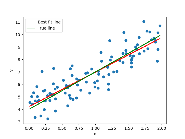
There’s some fake data in the file data.csv, with a single feature x and a true value y. Your task is to:
- Load the data and look at it
- Split it into training, validation, and test sets
- Create your design matrix
- Implement gradient descent to find the best fit polynomial
- Evaluate your model’s performance and experiment with different hyperparameters
It’s up to you to decide what degree polynomial to fit the data, and you can also play around with stochastic gradient descent, mini-batch, hyperparameters, etc.
Important
Do this without the use of scikit learn or other libraries aside from
numpyandmatplotlib!
Step 0: Import libraries and seed your random number generator
It’s usually a good idea to start with a consistent random number seed to ensure reproducibility.
import numpy as np
import matplotlib.pyplot as plt

rng = np.random.default_rng(seed="integer_of_your_choice")
Step 1: Load the data and look at it
x, y = np.loadtxt("data.csv", delimiter=",", skiprows=1, unpack=True)
#TODO: visualize
Step 2: Split the data
Weird numpy quirk: by default, a 1D array has a shape of (n,), but to behave as a proper vector, we need to convert it to be (n, 1). An easy way to do this is to pass np.newaxis as the second index when sampling your y data, e.g.:
n = len(y)
train_ids = rng.choice()
x_train, y_train = x[train_ids,], y[train_ids, np.newaxis]
Don’t worry about the x values for now, as we’ll be matrixifying them shortly anyway.
Step 3: Create your design matrix .
For the example given in class, the design matrix was simply a column of 1s concatenated with the feature vector, i.e.:
For this exercise, you probably want to fit a higher degree polynomial, so the design matrix will be something like:
where is the degree of the polynomial you want to fit. Try multiple degrees and see what gives the best results.
A note on scaling: the range of x values in this example is fairly small, but if you choose a high degree polynomial you will still end up with fairly different scales for your “features”. Consider normalizing each column of the design matrix (other than the first column accounting for the bias term), remembering to calculate your scaling parameters on the training data and apply them to the validation/test data.
Since you’ll be doing this twice (train/test), you might want to define a function to create the design matrix given a vector x and a degree d.
Step 4: Implement gradient descent
This has a number of sub components. First you’ll need to define your gradient function. For mean squared error, the gradient can be calculated as:
where is your design matrix, is the current parameter vector, and is the true target value.
It’ll also be useful to define the actual mean squared error to evaluate your model:
Now you can define your hyperparameters and run your gradient descent. For batch gradient descent, you’ll need to define:
- learning rate (usually in the range of to )
- stopping criterion (can just be a fixed number of iterations)
The general algorithm for gradient descent is:
- Start with a random
- Calculate the gradient for the current
- Update as
- Repeat 2-4 until some stopping criterion is met
You could also try mini-batch or stochastic gradient descent by adding an outer epoch loop if you want to get fancy.
Step 5: Evaluate your model’s performance and experiment
Now that you’ve computed a final estimate of , apply it to your test set to see how well your model performs, perhaps by plotting the data as well as the best fit curve. If it doesn’t look good, try changing various hyperparameters, like , number of iterations, and degree of polynomial. If you didn’t rescale your design matrix earlier, try it now!
Technically we should have done a 3-way train/validate/test split, but I kept it as just train/test to keep things manageable.
Backpropagation with a toy MLP
Before we move on to a full-featured toolbox, I wanted to provide you with something a bit simpler. I’ve written some (questionable) code in mlp_regressor.py to try to implement a multi-layer perceptron. I’ve also provided a starter notebook after throwing you to the wolves last week - you can download your copy here, or from GitHub.
Step 1: Load and preprocess data
We’ll use a well-known and fairly clean dataset to try to predict wine quality. You’ll still need to encode (or ignore) the one categorical feature color, then split and normalize the inputs. You’ll also need to pip install ucimlrepo to get the data-fetching module.
Step 2: Build and train an MLP
The MLPRegressor class should be able to train a small multi-layer perceptron. You can use it like this:
from mlp_regressor import MLPRegressor
mlp = MLPRegressor(X_train.shape[1])
mlp.add_layer(<number of neurons>, "activation function")
... repeat
print(mlp) # to see a summary of layers

loss = mlp.train(X_train, y_train, step_size, epochs)
plt.plot(loss)
It’s very inefficient, so don’t go too crazy with number of neurons. After training, you can predict by just running the forward pass:
y_pred = mlp.forward(X_train)
There’s also an example in the main block of mlp_regressor.py
Step 3: Modify the MLP
Try to read through the forward and backward passes to understand how it works. It’s entirely possible I’ve made a mistake somewhere, so don’t hesitate to ask if something doesn’t make sense.
To understand things in more detail, it can be helpful to try to modify it. Right now, the MLP only does whole-batch gradient descent. Can you modify it so that it does mini-batch or stochastic gradient descent?
Modern neural networks with PyTorch
In this lab, I’m going to be walking through the PyTorch intro code that we started in lecture before the midterm. This is a pretty small model so it should be feasible on lab computers or laptops, but you might want to get used to using Colab as well.
I’ll also introduce you to Assignment 2!
RNN Activity: Predicting the stock market
[!NOTE] I do not recommend making any kind of financial decisions based on RNNs.
Setup
To fetch the data, we’ll need the yfinance package. Activate your virtual environment, then run pip install yfinance. The starter notebook shows how to download some data.
Steps
- As usual, we need to split the data. For time series data, it is very important that you split chronologically, not randomly. The
yfinancedata has aDateTimeIndex, which means that we can index it with dates directly, e.g:
This also assumes that we’re interested in just the daily closing price. I’d suggest at least a year’s worth of data for both test and validation, with the rest for training.train_end = '2023-12-31' train = data['Close'][:train_end].values - Decide on a scaling factor and rescale your data to the 1-ish range. This should not be informed by the test or validation data!
- Follow the various TODO items to get the single-prediction RNN working.
- Modify both the
TimeSeriesDatasetand theSimpleRnnModelto predict multiple days in the future instead of just one.[!TIP] You may need to
squeezeand/orexpandyour data at some point in the process to ensure the data dimensions are correct
Further Exercises and Questions
- What impact does the scaling have on the model? Can you trigger exploding/vanishing gradients?
- Can you improve the model? Try playing around with LSTM/GRU instead of RNN, number of hidden units, activation functions, etc
- What happens if you pass a longer time window to the model? You will need to create a new
torch.FloatTensorfrom the numpy data to do this instead of using theTimeSeriesDatasetclass.
Tutorial 10: Applied Transformers
We don’t really have the computational resources to train our own transformer models, but we can play around with pre-trained models.
The HuggingFace Transformers API is an easy way to download a pre-trained model and either use as-is, or fine-tune for your application. I’ll provide a few suggestions, but the official tutorial has a lot more info.
Using pretrained transformer models
If you’re working on Kaggle or Colab, the transformers library may already be installed; otherwise, you’ll need to pip install transformers.
-
Pick a task and a model from the model list - I recommend sticking to something on the small side for your own sanity. Text generation is fun to play with so I’m going to start there, e.g.:
from transformers import pipeline

pipe = pipeline("text-generation", model="deepseek-ai/DeepSeek-R1-Distill-Qwen-1.5B")
Tip
If you’re on a GPU-enabled platform like Kaggle, you can move the model to GPU as follows:
from accelerate import Accelerator device = Accelerator().device pipe = pipeline("text-generation", model="deepseek-ai/DeepSeek-R1-Distill-Qwen-1.5B", device=device) -
Test it out! The simplest way to interact with a text generation model is to pass it a string:
pipe("What is the airspeed velocity of an unladen swallow?") -
Add context. Some of the models (like the Deepseek example) allow additional chat context, e.g.:
messages = [
    {"role": "user", "content": "What is the airspeed velocity of an unladen swallow?"},
]
pipe(messages)
How does this affect the value that is returned?
-
You can inspect and modify the configuration of the pipeline with the
pipe.generation_configobject. Try changing thetemperatureparameter and see how it impacts the results, e.g.:pipe.generation_config.temperature = 1.5I’d also recommend reducing the
max_new_tokensso that it runs faster and doesn’t ramble quite so much! -
To make a real interactive chatbot, create a sentinel loop that:
- prompts for input
- passes the input to the pipeline
- prints out the response
- concatenates the response with the previous messages
- prompts for input again
There’s lots more to play around with in this library, but that’s probably plenty for the tutorial time period.
Assignment 1: Data discovery and visualization
Due January 30, 2025 at 5 pm. Reasonable requests for extensions will be granted when requested at least 48 hours before the due date.
You may work in groups of 2 or 3. Click here to create your group on GitHub Classroom and clone the starting code.
Overview
Real world data is messy and incomplete in unexpected ways. Often, the information you need is in some kind of text field, or in a totally separate database that needs to be merged in. While I have done some basic filtering of the dataset, the focus of this assignment is on exploring and preparing the data for use with a machine learning model.
After exploring and cleaning your data, you will be training a regressor to predict a numeric value. You may choose any of the regression models from scikit-learn’s supervised learning modules, provided inference (prediction) is fairly fast (i.e. don’t use nearest neighbours). If you want to use something other than scikit-learn, just let me know - it’s probably fine! Again, the main focus of this assignment is the dataset exploration and processing part.
Choosing a model is a whole thing in itself, but don’t stress about it too much. Feel free to compare a couple, or consult this chart for guidance, but it doesn’t cover everything. Notably, decisions trees and random forests are missing, despite being pretty common, easily understood, and high-performing models.
I have set aside a subset of the data to test your model. Model performance will be evaluated and compared using the Mean Absolute Error. Note that since these are not practice or training datasets, the results may not be very good! As long as you’re in a reasonable range (less than about 100% relative error), your grade will not be affected by the prediction performance.
YYC Housing Data
Download the csv from Google Drive (it’s too big for GitHub!)
I have removed some redundant columns and excluded non-residential properties such as parking spots. I’ve also combined the 2023 and 2024 assessment values and excluded properties where the roll_number disappeared from one year to the next (e.g. in the case of a subdivision).
Unlike the California housing dataset example, this contains property details and assessed values for each individual house in Calgary. Your goal will be to try to predict the change in assessment value from 2023 to 2024 based on the other columns of the dataset. Be careful though - there are some weird city-specific codes in there. For example, the sub_property_use column contains the following codes:
| Code | Description |
|---|---|
| RE0100 | Residential Acreage |
| RE0110 | Detached |
| RE0111 | Detached with Backyard Suite |
| RE0120 | Duplex |
| RE0121 | Duplex Building |
| RE0201 | Low Rise Apartment Condo |
| RE0210 | Low Rise Rental Condo |
| RE0301 | High Rise Apartment Condo |
| RE0310 | High Rise Rental Condo |
| RE0401 | Townhouse |
| RE0410 | Townhouse Complex |
| RE0601 | Collective Residence |
| RE0800 | Manufactured Home |
Similarly, the land_use_designation refers to the city’s land use zones, which restrict the type of building that can be constructed on a given property. These zones are about to become much simpler, but for now the column exists in the dataset. It’s up to you to decide how (or if) to use it.
Feel free to get creative! Did odd-numbered houses increase more than even? Does distance from city centre make a difference? Apply your domain knowledge to select and transform your features.
Deliverables
Your assignment should consist of both a .ipynb notebook (committed with cells rendered) for your exploratory analysis and model training, as well as your “production” code providing a predict function.
Exploration and model training notebook
This notebook should follow the general process outlined in class to do the first four steps of the ML Project Checklist, plus training of a simple model. The emphasis is on the data exploration and preparation rather than the model itself. Model shortlisting and fine-tuning is not required (though it is allowed if you’d like).
Specifically, this notebook should include:
- loading the data
- setting aside a test set (as appropriate for the problem)
- exploratory visualizations, with comments about your observations
- your preprocessing pipeline
- your model training, either with cross-validation or a set-aside validation dataset
- saving your pipeline + model for production
Some guidelines are provided in the template notebook - feel free to modify as desired.
If you try something and then ultimately don’t use it, it’s fine to leave it in the notebook. I’d like to see things you thought of and then discarded.
Note
While most of your preprocessing decisions are up to you, please do not drop any samples. If you encounter missing values, you can drop the column or impute values, but the number of predicted values must match the number of input samples.
“Production” code
After deciding on a preprocessing pipeline, training a model, and saving it all to disk, implement the function predict in prod.py. This function should:
- load the required libraries
- load your model from disk
- apply your preprocessing
- return the predicted values
If you are using Scikit-learn’s Pipeline class to combine preprocessing with your regression model, then this function could be as simple as loading your pipeline and returning pipeline.predict(data).
predict should take as input a Panda dataframe of the data with the re_assessed_value_2024 column removed, and return a Numpy array of predicted property assessment changes from 2023 to 2024. Make sure not to drop any samples! The length of the output must match the length of the input.
Important
Make sure that I can run your
prod.pycode! I will be running your code from a master script in a Python 3.12 environment with the packages defined inrequirements.txtinstalled. I will alsocdto your repo and importprod. Please ensure:
- You are loading your model using a relative path
- If you have additional Python dependencies, add them to
requirements.txt- If you want to use a different language altogether, that is okay - just make sure that your dependencies are clearly documented and easy to install on Windows 11.
Written response
Answer the questions in README.md. Point form and short responses are fine! If you really hate Markdown, you can add a PDF instead.
Tips
-
I recommend creating a virtual environment and installing the packages in
requirements.txt. This will ensure that your code runs on my system:python -m venv venv pip install -r requirements.txton a Mac, use
python3andpip3instead.If you use any other packages and want to add them to the requirements list, you can update it with:
pip freeze > requirements.txt(again with
pip3if you are a Mac user). -
The end-to-end ML project from the textbook (presented in a condensed form in class) provides examples of some data transformation and visualization techniques, but these do not cover all scenarios. You may need to do some additional research to find the right technique for your dataset - in this case, make sure to cite your sources with a comment in your code.
-
I have reserved some data for a friendly competition between groups. You might want to test your
predictfunction with your own subset of data to make sure the loading and processing behaves in an isolated environment. -
Make sure to remove the target column from the dataframe before processing! I will be calling
predictwith a dataframe that hasre_assessed_value_2024removed.
Marking Scheme
Each of the following components will be marked on a 4-point scale and weighted.
| Component | Weight |
|---|---|
| Data exploration (visualizations, observations) | 30% |
| Preprocessing decisions | 30% |
| Model inference works and training approach is good | 20% |
| Written responses | 15% |
| Score | Description |
|---|---|
| 4 | Excellent - thoughtful and creative without any errors or omissions |
| 3 | Pretty good, but with minor errors or omissions |
| 2 | Mostly complete, but with major errors or omissions, lacking in detail |
| 1 | A minimal effort was made, incomplete or incorrect |
| 0 | No effort was made, or the submission is plagiarized |
Assignment 2: Playing card classification
Due March 6, 2026 at 5 pm, with the usual weekend flexibility.
You may work in teams of 2 or 3. Click here to create your team on GitHub Classroom and clone the starter code. This can be the same team or different from assignment 1.
Overview
The purpose of this assignment is to apply your theoretical knowledge of neural networks (particularly convolutional neural networks) to a real application. You will build and train a model from “scratch” (using PyTorch or some other framework, not really from scratch), and then see how much you can reduce its size while minimizing performance degradation. In addition to building and tweaking a neural network, this assignment serves as an introduction to:
- Working with a modern NN framework
- Preprocessing for image data
- Evaluating classification models
Dataset
This time, I’m choosing the dataset: Playing Cards. This is quite a clean dataset with reasonable class balance. There are lots of implementations of classifiers using this dataset, and if you do look at someone else’ work for ideas, make sure to cite your sources and understand what you are implementing.
Caution
This dataset is very consistent compared to playing cards found in the wild. I will be evaluating on my own hand-curated dataset - you may want to augment yours with some extra card images as well.
Deliverables
Your assignment should consist of the following:
- Your notebook(s) and/or Python scripts where you did your experiments, with the final training run and evaluation rendered
- A report describing your experiments and your final model decisions
- Your final model classes in a Python module named
your_team_name.py, alongside saved weights. Please make sure that your models load and run properly in Colab. If additional packages are required, list them in your report document.
I would recommend working in parallel with your teammate(s) and commit your changes after each experiment. It’s fine if you have multiple working notebooks, just indicate to me which is the final version.
Your training code
Your training code (notebook or Python script) should:
- Load the training data and do some basic data exploration, like looking at samples, number of classes, class distribution, etc. The code in
starter.ipynbprovides some ideas for connecting Colab to Google Drive, defining the training dataset, and inspecting a few samples. - Do any preprocessing you might want to do (at the very least, you’ll probably want to rescale the images from unsigned ints in the range 0-255 to floats in the range 0 to 1)
Hint: Pytorch has some preprocessing layers that you can stick on the start of your model much like Scikit-learn’s pipelines. Check out Torchvision Transforms for more ideas.
- Define and train a model, keeping in mind the following:
- The input layer must match the number of channels of your input. You do not need to define the batch size.
- The output layer must have as many neurons as classes you are trying to predict.
- Everything in between is a design choice that you can tweak!
- Iterate! I would suggest starting with a simple CNN feeding in to a fully connected output layer. I included my fairly random and not at all optimized model in the starter code.
- Train two models: one “best performance” version, where you try to get the highest accuracy, and one “size optimized” where you try to maintain reasonably good accuracy with the fewest parameters.
- Once you’ve trained your models, save the weights using
torch.save(model.state_dict())as described here. You may need to share these with me via Google Drive if they end up too big, but if not, you can just commit the binary weights file to your repo.
Your production code
To load the weights for your model and run inference, PyTorch needs to know the class definition. There is a way of saving the whole thing at once, but it’s fragile (much like pickling a Scikit-learn pipeline with custom functions).
After you’re happy with both small and large models, copy the class definitions in a Python module named for your team name (e.g. super_awesome_team.py). Also copy over your transformation pipeline - I will be passing this to ImageFolder when I load the top secret evaluation set. You can either use the same one for small and large models, or two separate ones, or parameterize with image size, etc.
from super_awesome_team import SmallModel, BigModel, img_transform
model = SmallModel()
model.load_state_dict(torch.load(path_to_small_weights, weights_only=True))
model.eval() # disables dropout and batch norm for inference
Tip
Make sure to include any necessary preprocessing like rescaling in your transformation pipeline, but do not include image augmentation steps like
RandomHorizontalFlip.
Your report
In a separate document, summarize your experiments, models, observations, reflections, etc. I’ve provided a template with more details in the starter code (report.md), though you aren’t limited to the markdown format.
Marking Scheme
Each of the following components will be marked on a 4-point scale and weighted.
| Component | Weight |
|---|---|
| Report: model development and experimentation | 20% |
| Report: reflections | 20% |
| Report: abstract and appendices | 20% |
| Model: load and run on Colab | 20% |
| Model: performance (highest accuracy model) | 10% |
| Model: performance / parameters ratio (size optimized) | 10% |
| Score | Description |
|---|---|
| 4 | Excellent - thoughtful and creative without any errors or omissions |
| 3 | Pretty good, but with minor errors or omissions |
| 2 | Mostly complete, but with major errors or omissions, lacking in detail |
| 1 | A minimal effort was made, incomplete or incorrect |
| 0 | No effort was made, or the submission is plagiarized |
Assignment 3: Classification of Text Data
Due March 20 27, 2026
You may work in teams up to 3. Click here to create your team on GitHub Classroom.
Overview
The purpose of this assignment is to further your hands-on experience in neural networks with a new type of data: text!
Dataset and task
Download the pre-split “Reddit jokes” csv here (200 MB). You will still need to do a validation split, but I’ve reserved a final test set as with the previous assignments.
The original dataset is 1 million reddit jokes, but I’ve modified it a bit. I added a threshold to the score value to classify each joke as is_funny = True or is_funny=False, and I’ve also removed some redundant columns. I left the score value in there so you can see just how “funny” people thought a given joke was, but the score cannot be used as a predictor.
Your task is to predict whether or not a joke is funny. You may use any of the information in the dataset except for the score column to predict the is_funny value.
[!WARNING] I have not vetted this dataset for appropriateness. While the “not safe for work” label is False for all features, there is still likely to be the usual degeneration one encounters on Reddit.
Many of the posts have [removed], [deleted], and NaN for the body text field. This is still information! Aside from replacing NaN with an empty string, you probably want to keep these features.
Deliverables
Your repo should have the following:
- Your notebook(s) and/or Python scripts where you did your experiments, with the final training run and evaluation rendered
- A report describing your experiments and your final model decisions
- An inference script with a
classifyfunction that loads your model, performs any preprocessing necessary on the list of titles given as inputs, then returns a list of booleans containing the predicted funniness. If your model file(s) is too big for GitHub, you may share a link to it on Google Drive.
Resources
GPU resources are a challenge, and potentially more important with text data. Here are a few options to consider:
- Kaggle provides 30 hrs/week of free GPU usage
- Colab provides a “pay as you go” tier, which is 14/month. I hate asking students to pay for things, but think of it like the cost of a textbook. I’m testing out the pay as you go option, and it seems to be using up credits at roughly 1.5/hr on a T4 TPU.
Your training notebook
I’ve included some sample code in the starter.ipynb to get you started. If you’re not using Colab and/or PyTorch, you might need to massage things a bit more (yes, this ends up being an inordinate amount of time in any data project).
Your inference script
This time, I’m asking that you implement an inference script similar to assignment 1 in prod.py. This should handle your data processing, model class definitions, loading the model weights, etc. You can assume that I will be loading the model weights from the working directory; please use relative paths to your weights file.
Your report
In a separate document, summarize your experiments, models, observations, reflections, etc. I’ve provided a template with more details in the starter code (report.md), though as usual you aren’t limited to the markdown format.
Marking Scheme
I’ll be marking each component on the usual 4-point scale and weighting as follows:
| Component | Weight |
|---|---|
| Model development and experimentation process | 30% |
| Model performance and compatibility | 20% |
| Report: reflections | 30% |
| Report: other stuff | 20% |
As usual, the raw performance doesn’t matter too much provided it behaves “okay”
| Score | Description |
|---|---|
| 4 | Excellent - thoughtful and creative without any errors or omissions |
| 3 | Pretty good, but with minor errors or omissions |
| 2 | Mostly complete, but with major errors or omissions, lacking in detail |
| 1 | A minimal effort was made, incomplete or incorrect |
| 0 | No effort was made, or the submission is plagiarized |
Journal Club
Your 10% journal club mark consists of two components:
- Reading each paper and participating in weekly discussions (5%)
- Reading a single paper more thoroughly and presenting that paper (5%)
The signup sheet is on D2L. You will need to be logged in to your MRU Google account to access it.
Presentation
The week you have signed up to present, read the paper and prepare a (maximum) 10 minute presentation. You may use whatever file format you wish, and feel free to copy and paste relevant diagrams or quotes from the paper (a single citation at the start suffices for this purpose). If you include material from other resources, these must be cited as usual.
When creating your presentation, consider the following guiding questions. You don’t need to use these headings specifically, and not every question applies to every paper, but it’s a place to start.
Paper Summary
- What are the main contributions of this work?
- What is the context (timeframe, prior knowledge, etc) of this paper?
- How did the authors justify their conclusions?
Paper’s influence
With the power of hindsight, we can look back and see what impact each paper had on the field of machine learning. Most of them are widely cited. Consider the following:
- If applicable, try to find implementations of the algorithms described by the paper. These may be shared by the authors (for more recent papers), or implemented by others (for pre-2000s papers)
- Are the methods described in the paper still relevant today?
- What is your impression of the impact that this paper had on the field of machine learning?
Your opinions
- What did you like about the paper?
- What was the most confusing or challenging to understand?
- Any additional thoughts?
Rubric
Each of the three sections will be assessed on a 4-point scale, with an additional score for sharing your thoughts and responding to classmates’ questions during the discussion period.
| Component | Score out of 4 |
|---|---|
| Paper summary | |
| Paper’s influence | |
| Your opinions | |
| Discussion | |
| Total out of 16 |
| Score | Description |
|---|---|
| 4 | Excellent - thoughtful and creative without any errors or omissions |
| 3 | Pretty good, but with minor errors or omissions |
| 2 | Mostly complete, but with major errors or omissions, lacking in detail |
| 1 | A minimal effort was made, incomplete or incorrect |
| 0 | No effort was made, or the submission is plagiarized |
Final Project: Predict something with some data
| Deliverable | Due date | Weight (of project) | |
|---|---|---|---|
| 1 | Proposal | Feb 27 Pitch Presentation in lab on March 2 | 15% |
| 2 | Checkpoint 1 | March 27 | 20% |
| 2 | Checkpoint 2 | April 13 | 20% |
| 4 | Final Report | April 24 Presentations on April 22* | 45% |
*I asked the registrar to schedule a block of time during final exams for you to share the outcomes of your projects, so this shows up on MyMRU as a final exam. You can put finishing touches on your report in the days afterwards.
You may work in teams of 2 or 3.
Overview
The goal of the final project is to showcase the skills you’ve learned in this course by applying them to a new dataset and task. You are free to choose anything you like, but do not pick a “hello-world” style dataset. I’d rather you take a risk and have it not be successful than recreate yet another Titanic survival prediction model.
Overall, throughout this project you will:
- Choose a task, such as classification, regression, time-series forecasting, NLP, etc.
- Find an appropriate dataset for that task. This is harder than it sounds, and may require some iterating when you start working with the data.
- Explore the data and preprocess as necessary to handle missing values, feature scaling, etc.
- Implement a model to accomplish your task.
- Write a formal report describing your project.
Tip
Often when you are writing a report and describing your methodology, you realize there is an error in that methodology and end up having to go back and fix something. Don’t leave the writeup to the very end - it’s a good idea to write as you go along.
Finding a Dataset
First, think of your interests and a possible prediction task, then look to see if there’s a relevant publicly accessible dataset. As you poke around you might do it the other way and stumble across an interesting dataset that inspires a task - that’s okay too!
Some good places to look for datasets:
- Hugging Face - A popular data- and model-sharing site, and the successor to the now-defunct “Papers with Code” (RIP)
- Google Dataset Search - of course Google does datasets as well.
- Wikipedia - a giant list of datasets for machine learning research.
- Google BigQuery Datasets - we’ll be using this in assignment 3, so I’ll provide guidance on accessing it
- Kaggle - a website for machine learning competitions with a huge number of datasets. You can filter by file size, topic and more
Submissions
This time, there is no starter code to share, as each of your projects will be different. Please submit your proposal, checkpoint and report as PDFs on D2L, and include a link to your code (e.g. on GitHub or Google Drive) in your final report abstract. This code may be public so you can use it as a portfolio piece, or if you prefer to keep it private, you can invite me to view it on GitHub.
4-Point Scale
Each of the components will be marked on various criteria using the usual 4 point scale. More details provided in each component description.
| Score | Description |
|---|---|
| 4 | Excellent - thoughtful and creative without any errors or omissions |
| 3 | Pretty good, but with minor errors or omissions |
| 2 | Mostly complete, but with major errors or omissions, lacking in detail |
| 1 | A minimal effort was made, incomplete or incorrect |
| 0 | No effort was made, or the submission is plagiarized |
Project Proposal
Your project proposal should be fairly concise, 1-2 pages consisting of the following sections.
Abstract
1-paragraph summary what you intend to do and with what data.
Project Plan
Using words, tables, images, etc, describe:
- The goal of your project
- The dataset you intend to use
- The approach you plan to take, referring to at least one paper
Risk Assessment and Backup Plan
Scoping a project is very challenging, and generally we want to do more than can be accomplished in the provided time. In this section, identify:
- Challenges you anticipate, and potential solutions/mitigations (this may be best presented as a table)
- A reduced scope goal that will still constitute project success if your primary objective can’t be met
References
Include a link to your proposed dataset and cite at least one technical paper describing the approach you plan to use.
Pitch Presentation
Prepare a very short presentation (1-2 slides, 3-4 minutes) to “pitch” your project during the lab on Monday, March 2. You can highlight whatever part is the most exciting to you, the main goal is to share with the class and learn who is working on similar projects.
Marking Scheme
Using usual 4 point scale, I will be assessing the following equally-weighted categories:
- Description of task and dataset
- Thoughtful risk assessment and contingency plan
- Appropriate references and tentative approach
- Pitch presentation
For a total of 16 points.
2. Checkpoint
At this point, you should have begun some preliminary data exploration and preprocessing. You may have also begun building your model pipeline. Your checkpoint report should again be 1-2 pages with the following sections:
Wins
What has been working so far? What are you excited about? Share your good news! This would be a good place to show some preliminary results or interesting data discoveries.
Challenges
What challenges (foreseen or otherwise) have you encountered? Is there anything in particular that you need help to get past?
Remaining work
What do you have left to do on your project? Is it feasible within the time constraints? If not, how do you plan to revise your project plan?
Project revision (if needed)
As a result of your progress to date, do you anticipate any changes to your project plan? It’s okay if it’s a significant change - perhaps you discovered a better dataset, or came up with a different approach.
If you do have major changes, please cite the relevant sources for your new revised project.
References
This section may not be necessary if you don’t have significant changes.
Marking Scheme
Using the usual 4 point scale, I will be assessing the following categories:
- Reasonable amount of progress made on project
- Description of challenges and assessment of progress
- Remaining work and revision (if needed)
- Overall coherence and clarity
For a total of 16 points.