Lecture 7: Convolutional Neural Networks
 HTML Slides
 PDF Slides
Convolution and Convolutional Neural Networks
COMP 4630 | Winter 2026 Charlotte Curtis
Overview
- Convolutional neural networks (CNNs) are a type of neural network that is particularly well-suited to image data
- Before we can understand CNNs, we need to understand convolution
- References and suggested reading:
- Scikit-learn book: Chapter 14
- Deep Learning Book: Chapter 9
- 3blue1brown video: What is convolution?
Convolution
-
Convolution is defined as:
-
Or in the discrete case:
-
Can be though of as “flipping” one function and sliding it over the other, multiplying and summing at each point
Example
We’re in a hospital dealing with an outbreak. For the first 5 days we have 1 patient on Monday, 2 on Tuesday, etc:
Fortunately, we know how to treat them: 3 doses on day 1, then 2, then 1:
And after 3 days they’re cured.
How many doses do we need on each day?
Convolution in 2D
- Extending to 2D basically adds another summation/integration:
- This can also be extended to higher dimensions
- Caution: a colour image is a 3D array, not a 2D array
- For typical image processing applications, the colour channels are convolved independently such that the output is still a 3D array
Convolution kernels
- Typically there is a small kernel that is convolved with the input
- This is just the smaller of the two functions in the convolution
- ❓ What happens at the edges of the input?

Some common kernels
- Averaging:
- Differentiation:
- Sizes are commonly chosen to be 3x3, 5x5, 7x7, etc.
- ❓ Why divide by 9?
- ❓ Why odd sizes?
- ❓ What effect do you think these kernels will have on an image?
A side tangent on frequency representation
- Any signal can be represented as a weighted summation of sinusoids
- For a discrete signal , you can think of this as:
- Or, using Euler’s formula : where the complex coefficients
Fourier Transform
- To figure out what the coefficients are, we can use the Discrete Fourier Transform (DFT): where each element of is the coefficient for frequency
- The Fast Fourier Transform (FFT) computes the DFT in time
- Convolution is
Convolution is multiplication in frequency
- Sometimes it is useful to use the Fourier Transform to obtain a frequency representation of an image (or signal)
- In the frequency domain, convolution is simply element-wise multiplication
- This allows for some efficient operations such as blurring/sharpening an image, as well as some fancy stuff like deconvolution
- Sharp edges in space become ringing in frequency, and vice versa
- ❓ why do CNNs operate in the spatial domain?
Convolutional neural networks
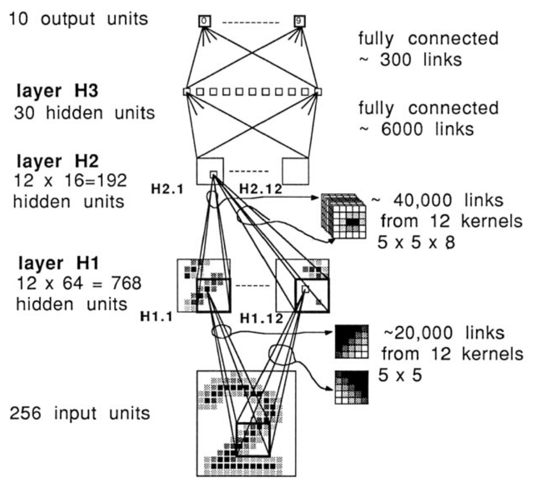
- 1958: Hubel and Wiesel experiment on cats and reveal the structure of the visual cortex
- Determine that specific neurons react to specific features and receptive fields
- Modelled in the “neocognitron” by Kunihiko Fukushima in 1980
- LeCun’s work in the 1990s led to modern CNNs
Why CNNs?
- A fully connected network has a 1:1 mapping of weights to inputs
- Fine for MNIST (28x28) pixels, but quickly grows out of control
- ❓ If you train a (fully connected) network on 100x100 images, how would you infer on 200x200 images?
- ❓ What if an object is shifted, rotated, or flipped within the image?

Convolutional layers
- A convolution layer is a set of kernels whose weights are learned
- Instead of the straight up weighted sum of inputs, the input image is convolved with the learned kernel(s)
- The output is often referred to as a feature map
- The dimensionality of the feature map is determined by the:
- Size of the input image
- Number of kernels
- Padding (usually “same” or “valid”)
- “Stride”, or shift of the kernel at each step
Dimensionality examples
| Input | Kernel | Stride | Padding | Output |
|---|---|---|---|---|
| 1 | same | |||
| 2 | same | |||
| 1 | valid | ??? |
- The number of channels has no impact on the depth of the output: the number of kernels determines the depth of the output
- The colour channels are convolved independently, then summed
Number of parameters example
- Input:
- Kernel:
- Bias terms: 32
- Total parameters:
While convolution only happens in 2D, the kernel can be thought of as a 3D volume - there’s a separate trainable kernel for each channel
Pooling layers
Pooling layers are used to reduce the dimensionality of the feature maps (aka downsampling) by taking the maximum or average of a region
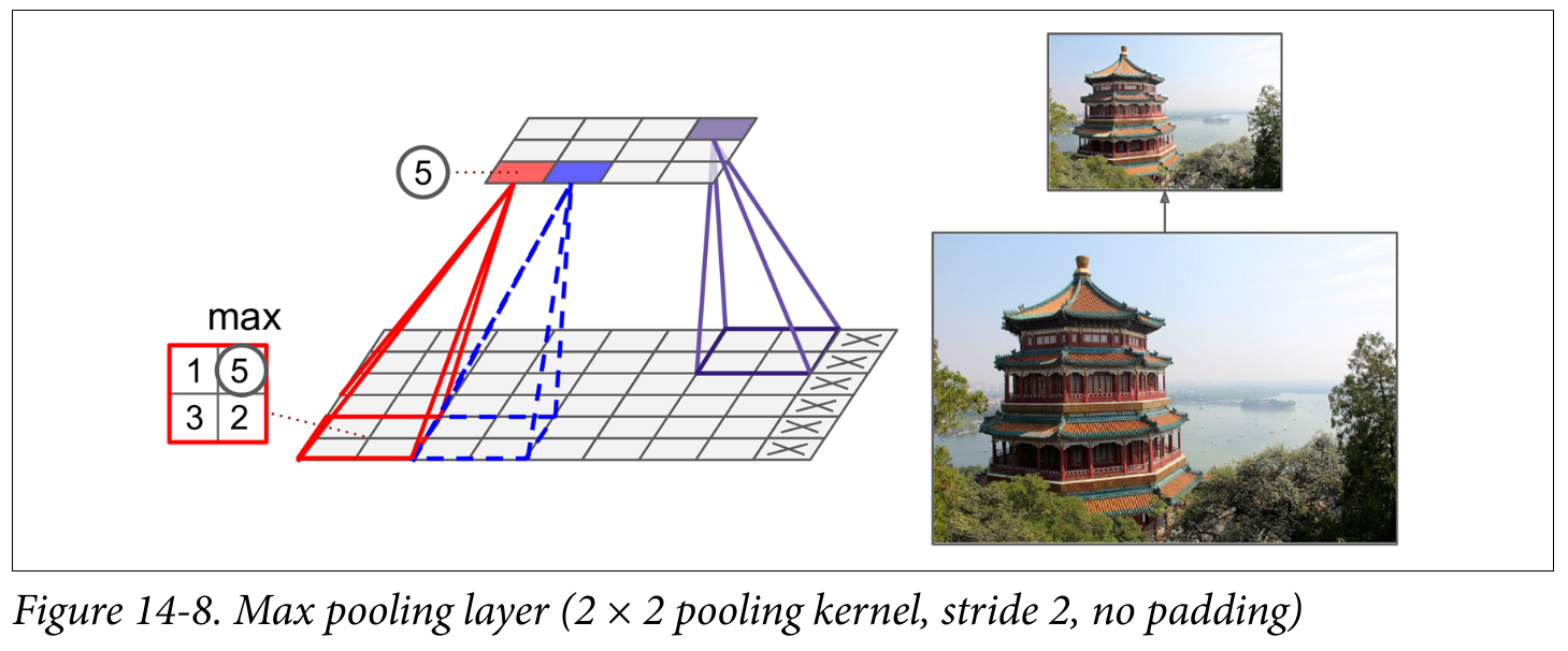
- ❓ Why would we want to downsample?
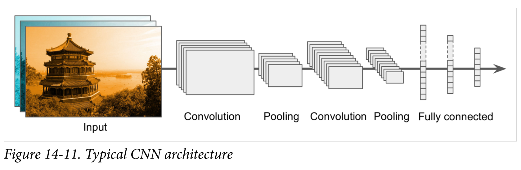
Putting it all together
Backpropagating CNNs
- After backpropagating through the fully connected head, we need to backpropagate through the:
- Pooling layer
- Convolution layer
- The pooling layer has no learnable parameters, but it needs to remember which input was maximum (all the rest get a gradient of 0)
- The convolution layer is trickier math, but it ends up needing another convolution - this time with the kernel transposed
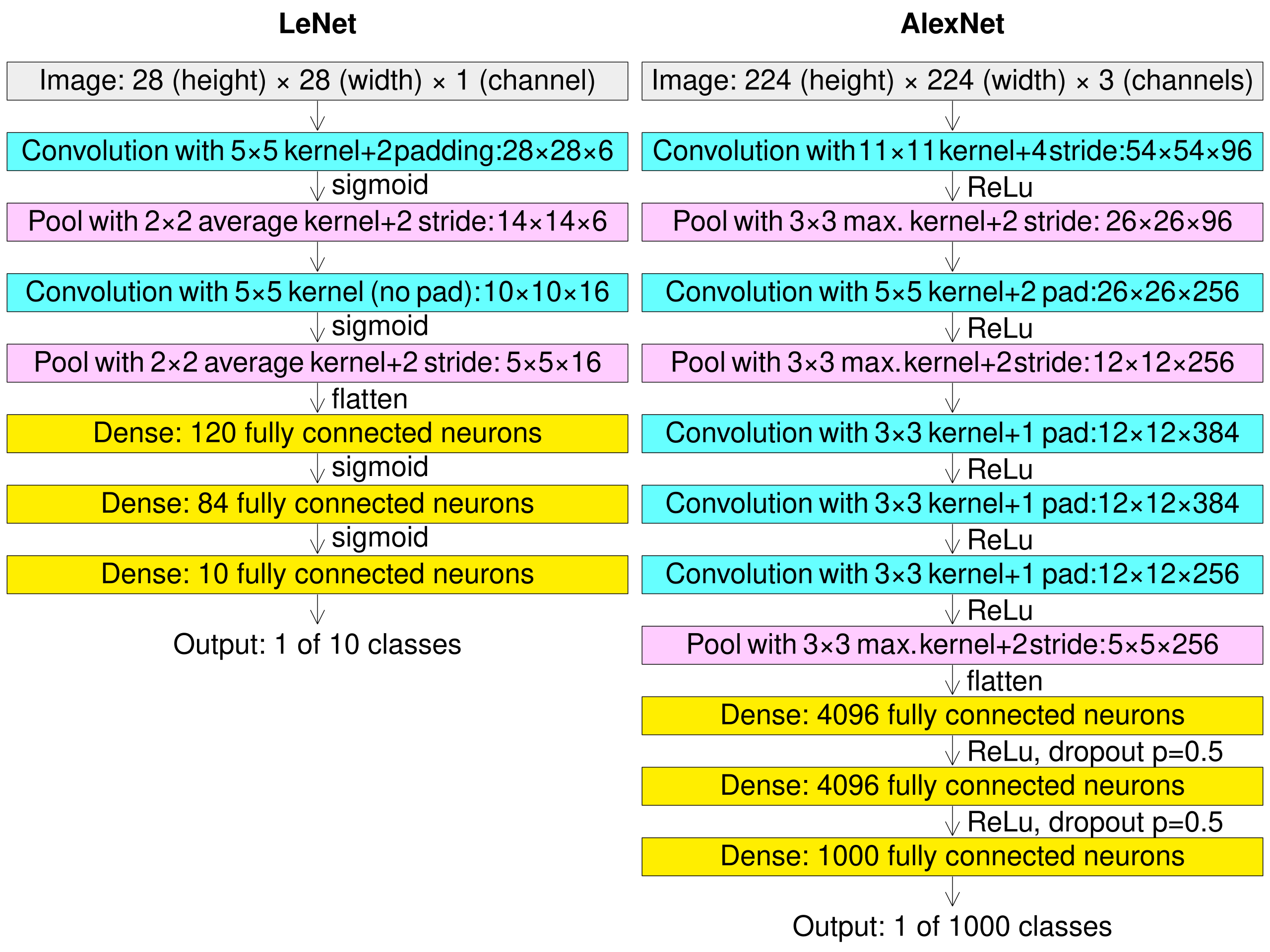
LeNet (1998) vs AlexNet (2012)
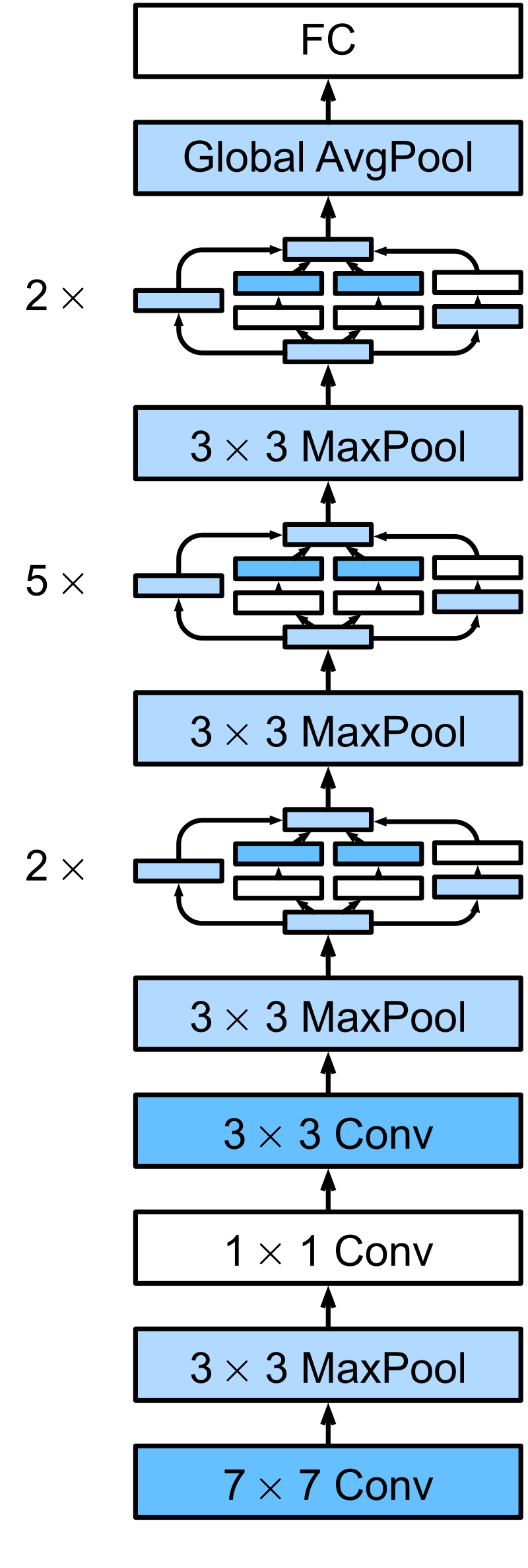
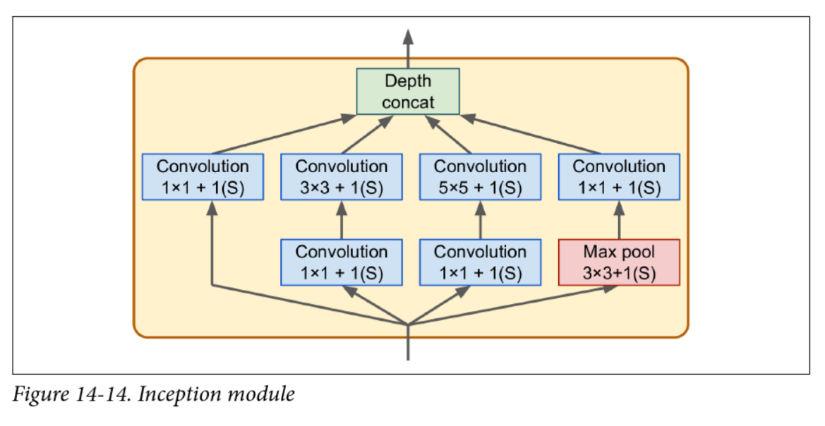
Inception v1 aka GoogLeNet (2014)
- Struggled with vanishing gradients
- v2 introduced batch normalization
VGG (2014)
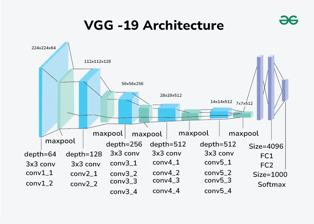
- Simple architecture, but “very” deep (16 or 19 layers)
- Fixed the convolution hyperparameters and focused on depth
ResNet (2015)
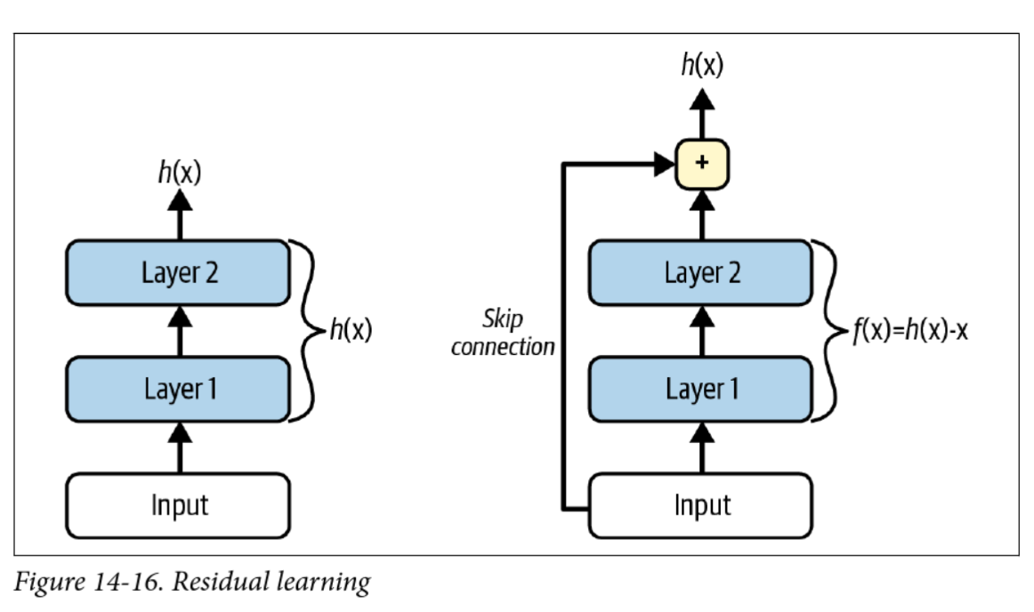
- Key innovation: easier to learn “identity” functions ()
- If a layer outputs 0, it doesn’t kill the gradient
- Even deeper, e.g. ResNet-152
Transfer Learning
“If I have seen further, it is by standing on the shoulder of giants” – Isaac Newton
- Transfer learning copy pastes a trained network into a new task
- You can select which layers to keep, which to freeze, and which to re-train
- You can also drop new layers on top of the old ones
- Most of the time you want to freeze the early layers and add a new “head”
Data Augmentation
-
Garbage in, garbage out
-
We can artificially increase diversity with data augmentation:
- Random crops, flips, rotations
- Rescaling/resizing
- Changing colours
-
AutoAugment does a bunch of this automatically