Lecture 4: Backpropagation
 HTML Slides
 PDF Slides
Backpropagation
COMP 4630 | Winter 2026 Charlotte Curtis
Overview
- A brief review of the history of neural networks
- Neurons, perceptrons, and multilayer perceptrons
- Backpropagation
- References and suggested reading:
- Scikit-learn book: Chapter 10, introduction to artificial neural networks
- Deep Learning Book: Chapter 6, deep feedforward networks
The rise and fall of neural networks

In between each era of excitement and advancement there was an “AI winter”
Model of a neuron
- McCulloch and Pitts (1943)
- Neuron as a logic gate with time delay
- “Activates” when the sum of inputs exceeds a threshold
- Non-invertible (forward propagation only)
Threshold Linear Units (TLUs)
- Linear I/O instead of binary
- Rosenblatt (1957) combined multiple TLUs in a single layer
- Physical machine: the Mark I Perceptron, designed for image recognition
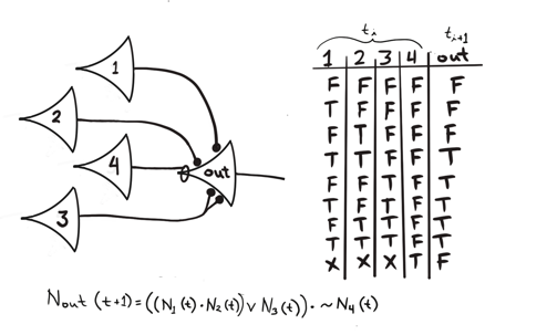
- Criticized by Minsky and Papert (1969) for its inability to solve the XOR problem - first AI winter
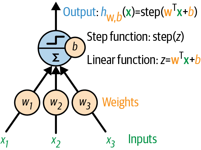
A single threshold logic unit (TLU)
Image source: Scikit-learn book
Training a perceptron
-
Hebb’s rule: “neurons that fire together, wire together”
where = input, = output
-
Fed one instance at a time,
-
Guaranteed to converge if inputs are linearly separable
-
:abacus: Simple example: AND gate
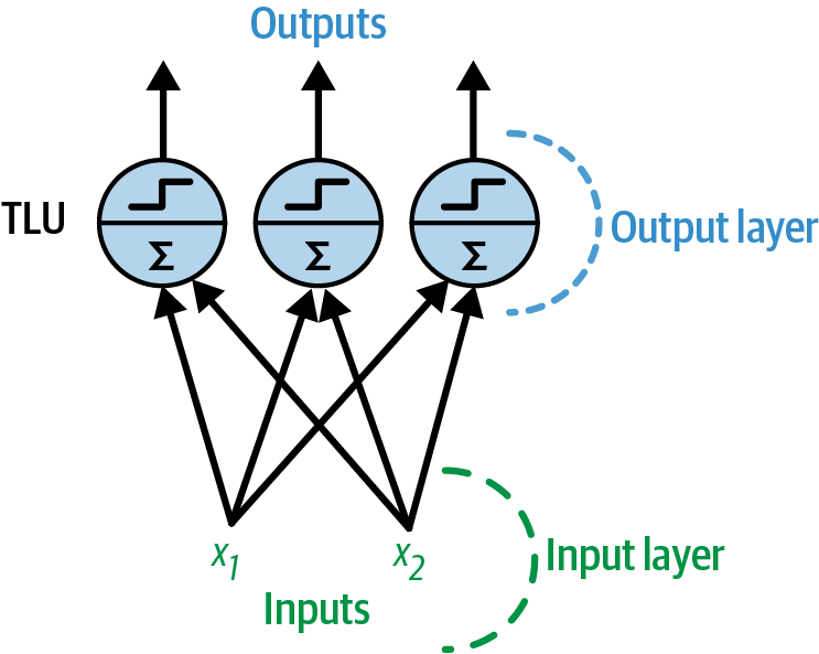
A perceptron with two inputs and three outputs
Image source: Scikit-learn book
Multilayer perceptrons (MLPs)
-
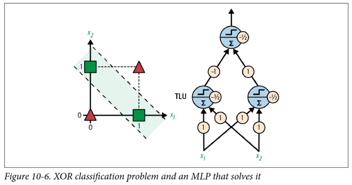
If a perceptron can’t even solve XOR, how can it do higher order logic?
-
Consider that XOR can be rewritten as:
A xor B = (A and !B) or (!A and B) -
A perceptron can solve
andandorandnot… so what if the input to theorperceptron is the output of twoandperceptrons?
A solution to XOR
Backpropagation
- I just gave you the weights to solve XOR, but how do we actually find them?
- Applying the perceptron learning rule no longer works, need to know how much to adjust each weight relative to the overall output error
- Solution presented in 1986 by Rumelhart, Hinton, and Williams
- Key insight: Good old chain rule! Plus some recursive efficiencies
Training MLPs with backpropagation
-
Initialize the weights, through some random-ish strategy
-
Perform a forward pass to compute the output of each neuron
-
Compute the loss of the output layer (e.g. MSE)
-
Calculate the gradient of the loss with respect to each weight
-
Update the weights using gradient descent (minibatch, stochastic, etc)
-
Repeat steps 2-5 until stopping criteria met
Step 4 is the “backpropagation” part
Example: forward pass
- With a linear activation function:
- In summation notation for a single sample:
- In this case,

and
Example: calculate error and gradient
- We never picked a loss function! Let’s assume we’re using MSE
- For a single sample: with the added for convenience
- The goal is to update each weight by a small amount to minimize the loss
- Fortunately, we know how to find a small change in a function with respect to one of the variables: the partial derivative!
Recursively applying the chain rule
-
Weights in the second layer (connecting hidden and output):
-
For the first layer (connecting inputs to hidden): where is the output of the hidden layer
Bias terms
- The toy example did not include bias terms, but these are very important (as seen in the perceptron examples)
- With a single layer we can add a column of 1s to , but with multiple layers we need to add bias at every layer
- The forward pass becomes:
- Or in summation form:
Gradient with respect to the bias terms
- For layer 2 (the output layer):
-
For layer 1:
where is the input to the hidden layer
Summary in matrix form
| Parameter | Gradient |
|---|---|
| Weights of layer 2 | |
| Bias of layer 2 | |
| Weights of layer 1 | |
| Bias of layer 1 |
Computational considerations
-
Many of the terms computed in the forward pass are reused in the backward pass (such as the inputs to each layer)
-
Similarly, gradients computed in layer are reused in layer
-
Typically each intermediate value is stored, but modern networks are big
Model Parameters Our example 6 AlexNet (2012) 60 million GPT-3 (2020) 175 billion
Choices in neural network design
Activation functions
-
The simple example used a linear activation function (identity)
-
To include other activation functions, the forward pass becomes:
-
The gradient in the output layer becomes: where , or the summation the second layer before applying the activation function
-
Problem! That step function in the original perceptron is not differentiable
Activation functions
- A common early choice was the sigmoid function:
- A more computationally efficient choice common today is the “ReLU” (Rectified Linear Unit) function:
Activation functions in hidden layers
The design of hidden units is an extremely active area of research and does not yet have many definitive guiding theoretical principles. – Deep Learning Book, Section 6.3
- Activation functions in hidden layers serve to introduce nonlinearity
- Common for multiple hidden layers to use the same activation function
- Sigmoid, ReLU, and tanh (hyperbolic tangent) are common choices
- Also “leaky” ReLU, Parameterized ReLU, absolute value, etc
- Can be considered a hyperparameter of the network
Loss functions
- The choice of loss function is very important!
- Depends on the task at hand, e.g.:
- Regression: MSE, MAE, etc
- Classification: Usually some kind of cross-entropy (log likelihood)
- May or may not include regularization terms
- Must be differentiable, just like the activation functions
Activation functions in the output layer
- Activation functions in the output layer should be chosen based on the loss function (and thus the task)
- Regression: linear
- Binary classification: sigmoid
- Multiclass classification: softmax (generalization of sigmoid)
- Again, must be differentiable
A complete fully connected network
